It is also possible to carry out simple thermodynamic cycle calculations with the
CoolProp classes. These calculations are based on the utility classes
CoolProp.Plots.SimpleCycles.StatePoint and
CoolProp.Plots.SimpleCycles.StateContainer, which can be used on their
own as demonstrated below. Note that the utility classes support numerous notations
to access their members and you can chose the one you like best or mix them:
In [1]: from __future__ import print_function

In [2]: import CoolProp

In [3]: from CoolProp.Plots import StateContainer

In [4]: T0 = 300.000; p0 = 200000.000; h0 = 112745.749; s0 = 393.035

In [5]: cycle_states = StateContainer()

In [6]: cycle_states[0,'H'] = h0

In [7]: cycle_states[0]['S'] = s0

In [8]: cycle_states[0][CoolProp.iP] = p0

In [9]: cycle_states[0,CoolProp.iT] = T0

In [10]: cycle_states[1,"T"] = 300.064

In [11]: print(cycle_states)
Stored State Points:
state        T (K)       p (Pa)    d (kg/m3)     h (J/kg)   s (J/kg/K)
    0      300.000   200000.000            -   112745.749      393.035
    1      300.064            -            -            -            -
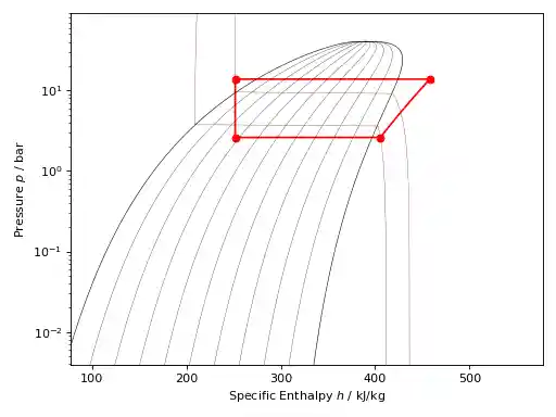
The utility classes were designed to work well with the plotting objects described above and this example illustrates how a simple Rankine cycle can be added to to a \(T,s\) graph, note how the unit conversion is handled:
import CoolProp
from CoolProp.Plots import PropertyPlot
from CoolProp.Plots import SimpleCompressionCycle
pp = PropertyPlot('HEOS::R134a', 'PH', unit_system='EUR')
pp.calc_isolines(CoolProp.iQ, num=11)
cycle = SimpleCompressionCycle('HEOS::R134a', 'PH', unit_system='EUR')
T0 = 280
pp.state.update(CoolProp.QT_INPUTS,0.0,T0-10)
p0 = pp.state.keyed_output(CoolProp.iP)
T2 = 310
pp.state.update(CoolProp.QT_INPUTS,1.0,T2+15)
p2 = pp.state.keyed_output(CoolProp.iP)
pp.calc_isolines(CoolProp.iT, [T0-273.15,T2-273.15], num=2)
cycle.simple_solve(T0, p0, T2, p2, 0.7, SI=True)
cycle.steps = 50
sc = cycle.get_state_changes()
pp.draw_process(sc)
import matplotlib.pyplot as plt
plt.close(cycle.figure)
pp.show()
(Source code, png, .pdf)