Detection of an Optical/UV Jet/Counterjet and Multiple Spectral Components in M84
Optical observations of resolved extragalactic jets date back nearly 100 years, to the observation of the 20″ long jet in M87 by Curtis (1918). Several ground-based observations of jet knots and hotspots (usually far from the host galaxy) have occurred in the intervening years, though they remain relatively rare (e.g., Cayatte & Sol 1987; Fraix-Burnet & Nieto 1988; Falomo et al. 2009). The launch of the Hubble Space Telescope (HST), which provides observations with sub-arcsecond resolution and lower backgrounds, added significantly to the number of optically detected jets, typically lower-power Fanaroff & Riley (1974) type I sources (FR Is)6 (e.g., Sparks et al. 1995, 1996; Martel et al. 1998, 1999; Scarpa et al. 1999; Floyd et al. 2006), where the synchrotron emission typically peaks at or just beyond the optical band. However, detections of resolved jets in the optical remain rare, with perhaps a few dozen detections in total. This is likely due to a combination of lack of observations (the vast majority of thousands of known radio jets have either never been observed with HST or lack deep observations) and the particularities of the broadband spectral energy distribution (SED) in some jets. In more powerful FR IIs, for example, it seems that the synchrotron peak is well below the optical, based on deep upper limits (e.g., Tavecchio et al. 2007) as well as very soft spectra in deep observations (Sambruna et al. 2006; Meyer et al. 2015; Breiding et al. 2017). This, in combination with the competition from host galaxy light in many cases, leads to very low detection rates. In consequence, the SEDs of most resolved jets are not measured at all beyond the radio, which means that it is difficult to assess theoretical models of jets on these scales or to quantify, e.g., the total energy they carry (with implications for jet feedback models).
With the launch of the Chandra X-ray Observatory in 1999 came the realization that many resolved radio jets produce significant X-ray emission, at kiloparsec distances from the bright “core” at the base of the jet (Chartas et al. 2000; Sambruna et al. 2002, 2004, 2006; Harris & Krawczynski 2006; Marshall et al. 2011; Kharb et al. 2012, and many more). Well over 150 sources have been detected, including both jets and terminal hotspots.7 In many cases, the X-ray emission from the kiloparsec-scale jet is both much harder and far above what is expected from the radio–optical synchrotron spectrum, indicating a second emission component, leading to their sometime designation as “anomalous” X-ray jets. For many years, the preferred explanation for the anomalously high X-ray flux (found in mostly powerful FR IIs) has been inverse Compton upscattering of the Cosmic Microwave Background (IC/CMB) by a jet that remains highly relativistic on kiloparsec scales (Tavecchio et al. 2000; Celotti et al. 2001). However, this explanation predicts a well-defined, very high level of gamma-ray emission (Georganopoulos et al. 2006), which has subsequently not been seen in several cases (Meyer & Georganopoulos 2014; Meyer et al. 2015, 2017; Breiding et al. 2017). The model, which requires that the knots of the jets are moving “packets” of plasma, has also been ruled out in 3C 273 on the basis of stringent upper limits on the optical proper motions (Meyer et al. 2016) and in PKS 1136–135 based on the high degree of polarization in the UV portion of the second component (Cara et al. 2013). The IC/CMB model is also at odds with a number of observed properties of Chandra-detected jets, for example, the observed variability (Marshall et al. 2010) and jet-to-counterjet flux ratio in Pictor A (Hardcastle et al. 2016), offsets between radio and X-ray emission and the jet-to-counterjet flux ratio in 3C 353 (Kataoka et al. 2008), as well as the offsets between radio and X-ray knots in 3C 111 (Clautice et al. 2016), among others.
With the IC/CMB model now in serious doubt, remaining alternatives to explain the X-rays are few. In one of the papers announcing the discovery of the very first anomalous X-ray jet, PKS 0637–752, Schwartz et al. (2000) ruled out synchrotron self-Compton and thermal bremsstrahlung as possible mechanisms to produce the X-rays, with the former requiring gross departures from equipartition and unrealistic beaming parameters to match the X-ray flux, and the latter requiring unreasonably high electron densities that exceed limits implied by rotation measure studies (a similar result is found in this paper and in Harris et al. 2002 for M84). However, a second synchrotron spectrum has long been considered a possible explanation for the X-rays (Atoyan & Dermer 2004; Harris et al. 2004; Kataoka & Stawarz 2005; Hardcastle 2006; Jester et al. 2006; Uchiyama et al. 2006), with the main detraction being the unexpected and unexplained additional electron energy distribution required. Hadronic emission models are also a possibility (Aharonian 2002; Kusunose & Takahara 2017; Petropoulou et al. 2017), though they have not been extensively explored in this context.
While the debate over the X-ray emission has unfolded, it has also become apparent that many jets show a hardening of the spectrum in the optical/UV, either alone or apparently connected to the X-ray flux (as in 3C 273). In many cases, these UV and/or X-ray components cannot be consistent with IC/CMB, simply due to their spectral shape. The IC/CMB flux must be extremely Doppler boosted (δ ∼ 10–15) to reach the observed flux levels in the UV through X-rays, which implies that the spectral index should be equal to that in the low-frequency radio. This is often found to not be the case. Further, the UV and/or X-ray emission, under the IC/CMB model, comes from very low-energy electrons, which in turn implies extreme fluxes from the “peak” of the electron distribution at higher energies, which often overpredict either the X-rays (for UV components) or gamma-rays (for X-ray-detected components). Very hard second components have been found emerging in the UV with no or very low/soft X-ray emission, which is again not expected under an inverse Compton scenario—for example, in the inner knots of PKS 2209–089 (Breiding et al. 2017) and the outer knots of 3C 273 (Jester et al. 2006). A slight hardening of the X-ray spectrum in the inner knots of low-power jets like M87, 3C 346, and 3C 120 (Wilson & Yang 2002; Harris et al. 2004; Worrall & Birkinshaw 2005) also suggests a second component, though much less dominant than that found in powerful quasar jets.
As we present in this paper, the resolved jet in the radio galaxy M84 has three distinct components in the jet SED and is perhaps the best case of a low-power FR I with a separate X-ray component. As in Breiding et al. (2017), we propose the term “Multiple Spectral Component,” or MSC, jets for this broad class of objects where secondary (or tertiary) components are found, rather than the former “anomalous X-ray jet” usage. In general, these secondary and tertiary components are so far unexplained.
M84 is a very well-studied galaxy, being one of the four prominent ellipticals in the Virgo cluster (z = 0.00339, D = 18.5 Mpc), all of which are associated with hot X-ray gas (∼107 K, Forman et al. 1984) within an intracluster gas of somewhat higher temperature (∼3.5 × 10⁷ K). M84 hosts a weak FR I-type radio jet, along with a counterjet of nearly the same length and luminosity, suggesting a source that is nearly in the plane of the sky. The black hole at the center of M84 is relatively massive for the general AGN population, but in keeping with the higher masses typically seen in FR I-hosting ellipticals, at  (Walsh et al. 2010). Optically, the nucleus is classified as a LINER (Ho et al. 1997), and the jet and surroundings have been extensively studied in the radio and X-rays. Laing & Bridle (1987) mapped the Faraday Rotation across the M84 jet, finding that the rotation is due to gas in front of the radio lobes. The Chandra images show that the radio lobes occupy lower-density “cavities” within the X-ray-emitting gas (Finoguenov & Jones 2001; Finoguenov et al. 2008), with the southern jet totally contained by the X-ray gas, as evidenced by the “shell” features seen in the radio (Laing et al. 2011), while the northern jet is breaking free. X-ray emission coincident with the radio jet was first detected in Chandra imaging by Harris et al. (2002); the source was subsequently included in two surveys of X-ray jets (Massaro et al. 2011; Harwood & Hardcastle 2012), but no previous detection of the jet outside of the radio and X-ray bands has been reported.
In this paper, we report the detection of M84 in the optical and UV in archival HST imaging and in the submillimeter in archival ALMA observations. We also analyze many archival radio observations with the Very Large Array (VLA), both to measure the jet SED and to look for proper motions of the jet. In combination with a reanalysis of three separate Chandra observations of M84, we investigate the broadband SED of M84 for the first time and examine possible theoretical explanations for the unusual three-component SED, including hadronic models. In this paper, we use the spectral index convention fν ∝ ν−α and an angular distance scale of 89 pc arcsec−1 for M84.
2.1. Hubble Space Telescope
M84 has been observed by several of the instruments on HST as part of projects focused on science other than the radio jet. We first noticed the jet in the far-UV (F225W) WFC3 imaging during an archival search for optical counterparts to resolved jets detected by Chandra. The jet is most obvious in the UV because the competition from galaxy light is considerably less (the uncertainty in the galaxy subtraction is the reason for the larger error bars with the optical filters as described below); however, it is detected in all of the deep imaging we examined, summarized in Table 1.
Table 1. HST Observations
| Instrument | Filter | λc | Freq. | Exposure | Date | PID |
|---|---|---|---|---|---|---|
| (Å) | (GHz) | Time | ||||
| ACS/WFC | F850LP | 9036 | 2 × 560 s | 2003 Jan 21 | 9401 | |
| ACS/HRC | F606Wa | 6060 | 3 × 782 s | 2002 Dec 17 | 9493 | |
| ACS/WFC | F475W | 4745 | 2 × 375 s | 2003 Jan 21 | 9401 | |
| WFC3/UVIS | F336W | 3354 | 4 × 600 s | 2009 Nov 24 | 11583 | |
| 4 × 600 s | 2010 Mar 29 | 11583 | ||||
| WFC3/UVS | F225W | 2359 | 8 × 600 s | 2009 Nov 23–24 | 11583 |
Note.
aPolarization imaging.Download table as: ASCIITypeset image
We first analyzed the ACS/F475W data to produce a reference image. This filter was best suited for this purpose, since far more point sources are detected in the optical than UV, while the blue filter offers a slightly better PSF than the long-pass optical imaging. The F475W data were taken in a single visit, and we used the AstroDrizzle package to stack the two exposures into the final image using default parameters and a 0 04 final pixel scale. Given the low redshift of M84, the galaxy is quite large in angular extent and covers a large fraction of the HST detectors. To prepare a suitable reference image against which to align the other HST data (particularly the UV where the galaxy is barely detected), we modeled and subtracted the galaxy using the IRAF tasks ellipse and bmodel, and rotated the image into a north-up orientation.
Both UV data sets consist of two orbits (in the case of the F336W filter data, in two separate visits separated by four months). In order to best align the UV data to the F475W reference image, we ran AstroDrizzle on the two epochs separately. We again used default parameters other than a final pixel scale of 004. These individual images were then matched to the reference frame using the large number of point sources in each. This was accomplished using an approach very similar to that presented in Meyer et al. (2015) to align the multiepoch HST imaging of 3C 273. Briefly, we first made a rough alignment by hand-selecting five to six point sources common to the two images and calculating the best-fit six-parameter linear transformation. With a starting rough match, we were able to identify (again by eye) several more sources in common between the UV and reference images, including resolved background galaxies. There were 18 in the F225W images and 57 in the F336W images. By selecting a region of pixels covering each point source (about 1000 pixels per source), we found the optimal shift to match the reference image source to the UV image (after scaling the flux scale of the image to roughly match the reference image; see Meyer et al. 2015). These shifts were used to iteratively improve the six-parameter linear transformation best fit until no improvement in the rms of the shift values occurred. The final rms error on the background source positions was ∼0.2 pixels (8 mas) and ∼0.08 pixels (3 mas) using 14 and 14 final sources in the two epochs of F225W imaging and 40 and 47 in the F336W imaging. The final numbers of background sources were after rejecting outliers, some of which could be due to nonnegligible motion of foreground stars over the six years between the reference and UV imaging or residual cosmic-ray artifacts in the drizzle images. For each UV filter, the two epochs were combined using a simple averaging of the two images.
The ACS/F850LP data were matched to the reference image using nearly the same procedure as described above. While galaxy subtraction was not necessary prior to matching the UV data, the galaxy is extremely dominant in the F850LP imaging, and differences between the flux profile in the F850LP/F475W nonsubtracted images could affect the calculation of optimal position shifts. We thus modeled the galaxy in the initial F850LP drizzle image using GALFIT in order to produce a subtracted image both for calculating the alignment and producing the final rotated/matched image. The galaxy was well fit (with a final χ2 value of 0.231) with three Sérsic components with effective radii of 840, 177, and 64 pixels and indices of 1.00, 1.32, and 0.041 respectively.8 The two smaller Sérsic components had both mode 2 and mode 4 Fourier components, while the largest Sérsic index was slightly boxy (boxyness parameter 0.0483). The F850LP imaging consists of a single visit and was matched to the reference image with 58 initial reference sources. The final rms error in the registration is 0.084 pixels or 3 mas, using 26 final reference sources.
We also analyzed a relatively shallow ACS/HRC F606W polarization observation to look for signs of the polarization signature one might expect from synchrotron emission. Unlike the deeper imaging, these data were simply stacked into individual polarization filter images using AstroDrizzle and combined using the standard formulae (Kozhurina-Platais & Biretta 2004) to produce a total linear polarization image. The World Coordinate System parameters of all final images were made consistent using a large number of common background sources and the IRAF tasks ccmap and ccsetwcs.
Prior to the final scaling of the images for analysis, the F225W, F336W, and F475W images were all galaxy-subtracted. The model in the F475W filter was very similar to that of the F850LP image, with three Sérsic components with effective radii of 850, 185, and 66 pixels and indices of 1.00, 1.29, and 0.047 respectively. The two smaller Sérsic components had both mode 2 and mode 4 Fourier components, while the largest Sérsic index was slightly boxy (boxyness parameter 0.0382). The galaxy is much fainter in the UV images, so the fitting is less complex. The F225W model required only one Sérsic component, with a radius of 360 pixels and an index of 2.92, to reach a reduced-χ2 value of 0.918. For the F336W model, three Sérsic components were used, with radii of 616, 165, and 65 (indices of 1.09, 0.84, and 0.59), but no other shape parameters, resulting in a reduced-χ2 value of 0.104.
In Figure 1, we show the HST imaging, with the left panels prior to subtraction and the right panels after the subtraction, labeled with the appropriate filters. The overlaid contours are from the C-band VLA observation described below. We note that the jet is clearly seen in the optical in the first three filters, while in the F850LP filter the morphology appears somewhat unclear. While there is a statistically significant flux in the knot B region in this filter, it is not certain that the measured flux is correctly identified as coming from the synchrotron jet emission. However, this data point is not critical for any of the conclusions in this paper.
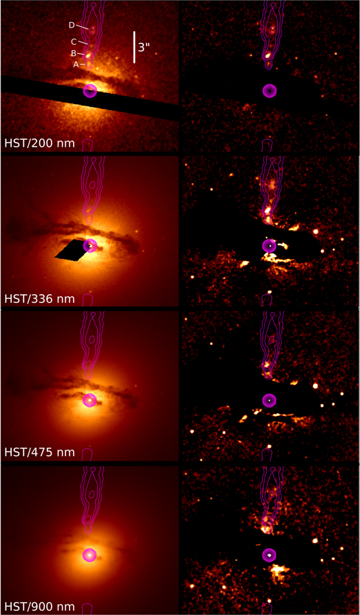
Figure 1. HST imaging of M84. In all cases, the left image is prior to galaxy subtraction and the right is after (postsubtraction images have been smoothed with a three-pixel Gaussian kernel). From top to bottom, the camera/filter is WFC3/F225W, WFC3/F336W, ACS/WFC/F475W, and ACS/WFC/F850LP. Radio contours are from the C-band image, with the first level starting at 180 μJy and subsequent levels increasing by factors of 2. Four of the radio knots are clearly seen in the UV image as indicated at the top panel, with the knots labeled A–D. The data used to create this figure are available.
Download figure:
Standard image High-resolution image
2.2. Very Large Array
We analyzed archival high-resolution C- and X-band observations of M84 to best match the HST resolution for measuring individual knot fluxes. The C-band observations were taken in A-configuration on 2000 November 18 as part of project AW0530, with 27 antennas, 200 MHz bandwidth, and 430 minutes on source over 10 hours, producing excellent UV coverage. The data were reduced using CASA version 4.7.38348-REL (r38335). After minor flagging of radio frequency interference, a standard calibration was applied, with 3C 286 as the amplitude calibrator and M84 itself serving as the phase calibrator. Several rounds of phase-only and a final round of amplitude and phase self-calibration were applied before producing the final image. The final image, shown on the left in Figure 2, has an rms of 22 μJy and a synthesized beam size of 043 × 041.
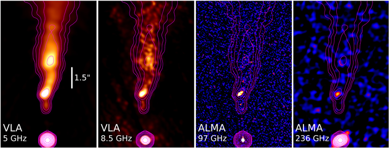
Figure 2. From left to right, the VLA C-band and X-band images of M84, followed by the ALMA band 3 and band 6 images. All have C-band radio contours overlaid as in Figure 1. For the ALMA images, the pixel scale is 5 and 20 mas, respectively, and the images have been smoothed by a Gaussian of width 10 pixels. The data used to create this figure are available.
Download figure:
Standard image High-resolution image
The X-band data were taken in A-configuration on 1999 September 05 as part of project AN8500, with 27 antennas, 200 MHz bandwidth, and 10.4 minutes on source. The analysis was similar to the C-band data with 3C 286 again as amplitude calibrator. The final self-calibrated image has an rms of 97 μJy and synthesized beam size of 025 × 022.
2.3. Jet-to-counterjet Ratios
In addition to the above, we used lower-resolution archival VLA data in the L, C, X, and Ku bands to study the jet-to-counterjet ratio. These were an L-band, A-configuration data set from 2015 July 03 (project 15A-305); a C-band, C-configuration observation from 2000 June 04 (project AW0530); an X-band, C-configuration observation from 1998 November 28 (project AR0402); and a Ku-band, D-configuration observation from 2015 December 20 (project BH212). The L- and Ku-band observations were calibrated using the JVLA pipeline, while the C- and X-band data were calibrated and flagged by hand. All were imaged using clean in CASA 4.7.2 using standard procedures, including self-calibration.
The reason for using lower-resolution imaging for the counterjet analysis was to avoid problems with missing flux due to the lack of short baselines in the A-configuration, especially at higher frequencies. The resolution of the images was on the order of 13, 35, 21, and 46, and the largest angular scale was on the order of 36″, 240″, 145″ and 97″ in the L, C, X, and Ku bands, respectively.
2.4. VLA Proper Motions with WISE
Two additional VLA observations were reduced to look for proper motions of the knots. Both were in C-band, A-configuration to match the resolution of the previous two high-resolution images. These were taken in 1984 December 09 (project AH167) and 1988 November 23 (project AW0228). These were reduced in the same manner as the epoch 2000 data, and all were put on an aligned coordinate system with a 20 mas pixel scale. We attempted to use similar-resolution archival data at higher frequencies, but none of the observations resulted in good detection of the jet features, due to the short observing times.
To look for proper motions of the knots, we used the publicly available Wavelet Image Segmentation and Evaluation (WISE) code (Mertens & Lobanov 2015; Mertens et al. 2016). The WISE code comprises three main components. First, the detection of structural information is performed using the segmented wavelet decomposition method. This algorithm provides a structural representation of astronomical images with good sensitivity for identifying compact and marginally resolved features and delivers a set of two-dimensional significant structural patterns (SSPs), which are identified at each scale of the wavelet decomposition. Tracking these SSPs detected in multiple-epoch images is performed with a multiscale cross-correlation algorithm. It combines structural information on different scales of the wavelet decomposition and provides a robust and reliable cross-identification of related SSPs.
The final reported proper-motion values given in Section 3.5 were obtained using a scale factor of 12 (for knot B) and 16 (for knot A), as these were the scales that yielded a good detection of each knot as a single component across multiple epochs. The fainter knots C and D in the jet were not consistently identified with a single feature and could not be tracked with the limited epochs available.
2.5. ALMA
We searched through the available ALMA archival data on M84; none of the observations available at the current time were taken with the goal of imaging the jet. However, the brightest knot in the jet (knot B) is detected in the band 3 and 6 imaging we present here.
The ALMA band 3 observation of M84 was taken as part of cycle 3 project 2015.1.01170.S where M84 served as a phase calibrator. The nominal resolution and largest angular scale is 006 and 055, respectively. We used CASA pipeline version 4.5.1 to produce the initial calibrated measurement set, while CASA version 4.7.1-REL (r39339) was used for self-calibration and imaging with clean. The observation included 240 scans on M84 for a total time on source of 72 minutes. After several rounds of self-calibration, the final imaged was produced, with an rms of 9 μJy and synthesized beam size of 006 × 005.
For the ALMA band 6 image, we used an observation from cycle 2 project 2013.1.00828.S (focused on measuring central black hole masses in AGN) where M84 was one of the targets. The observations have nominal resolution and largest angular scale of 034 and 174, respectively. We used the CASA pipeline version 4.3.1-REL (r32491) to produce the initial calibrated measurement set, while CASA version 4.7.1-REL (r39339) was used for self-calibration and imaging with clean. The observation included 12 scans on M84 for a total time on source of 49 minutes. After several rounds of self-calibration, the final imaged was produced, with an rms of 40 μJy and synthesized beam size of 029 × 021.
The VLA and ALMA images are shown in Figure 2, with C-band contours overlaid. While there is some hint of increased brightness in the overall inner -jet region in the band 3 image, only knot B is clearly detected in both ALMA images. In order to assess the effect of the minimum baseline on the largest resolvable scale, we used the Gaussian fit feature in CASA on knot B in the higher-resolution X-band image, which gives a resolved size of 0.6 ± 005 × 0.3 ± 005 for the knot. The band 6 ALMA image has a similar resolution to the X-band VLA image and finds a size of 0.35 ± 008 × 0.21 ± 003, suggesting the knot may decrease in size with increasing frequency. We thus do not expect a significant loss in the flux measurement in the ALMA imaging due to the short baseline limit of the observation, based on comparison to the largest angular scales, above.
2.6. Chandra
We analyzed three archival Chandra observations of M84 taken with ACIS-S, having IDs 803, 5908, and 6131 (taken on 2000 May 19, 2005 May 01, and 2005 November 07, respectively). These observations were obtained to study the interaction between the large-scale radio jet and the intercluster medium (Finoguenov & Jones 2001, 2002; Finoguenov et al. 2008). Harris et al. (2002) published an initial analysis of the M84 jet (finding two jet features) based on the first epoch of Chandra observations in 2000, with subsequent analyses using all three epochs by Massaro et al. (2011) and Harwood & Hardcastle (2012), reporting three and two distinct jet features, respectively. However, both of these later analyses of M84 were part of a much larger study of several dozen jets, and a necessary level of specificity in how the jet regions were selected is not available. To be certain that we measure the X-ray flux of the same regions we identified in optical and radio imaging, we have reanalyzed the M84 data.
The data were analyzed using CIAO version 4.9. For each epoch, we first ran the chandra_repro script to generate level 2 event files with the latest calibration applied. We made an initial energy selection of 0.4–8 keV in keeping with the standard practice of cutting out the parts of the observing window with a high background, and we included only data from the S3 chip. We then used the lc_clean script to remove background flares, resulting in final exposure times of 23.545, 45.311, and 36.834 ks for the three epochs, respectively.
We divided the jet into four regions, corresponding to knots A−D, as shown in Figure 3. A background region was carefully chosen to approximate the level around the jet region (shown to the right of the jet). The background is complicated by the fact that the environment of the jet has a strong thermal signature. We extracted counts from the same region in each epoch for analysis with sherpa. Before analyzing the individual regions, we first fit the entire jet area to increase the statistics for measuring the spectral parameters. We note here that no variability in the jet between epochs was observed, so we combined all observations in our analysis using standard methods. The model we used is a simple power law for the jet components, with a thermal plasma emission model (APEC) for the background. The details of the fits are given in Table 2, where we give the (fixed) galactic hydrogen value according to the mean value for the position in the online nH tool,9 the reduced statistic for the fit, the fixed redshift for the background thermal model, and other important parameters for the APEC and power-law models.
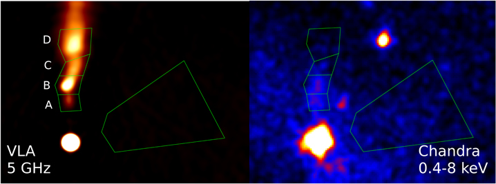
Figure 3. At left, the 5 GHz VLA image of M84 with the Chandra regions overlaid. The Chandra merged subpixel image (0.4–8 keV) with an exactly matching scale is shown at right, with the same regions overlaid. The large area to the right was used to estimate the background contribution, avoiding the non-jet related sources in the region. The data used to create this figure are available.
Download figure:
Standard image High-resolution image
Table 2. Chandra Spectral Fitting Results
| APEC Model | Power -law Model | ||||||||
|---|---|---|---|---|---|---|---|---|---|
| Component | gal. nH | Red. χ2 | z | Z a | kT | norm. | Γ | norm. | f0. 4–8,keVb |
| ×1022 cm−2 | keV | ×10−5 | ×10−7 | erg s−1 cm−2 | |||||
| Entire jet | (0.026) | 0.65 | (0.003392) | (0.3) | 0.72 ± 0.03 | 2.2 ± 0.1 | 2.0 ± 0.2 | 18.0 ± 3.1 | 8.6 × 10⁻¹³ |
| Knot A | (0.026) | 0.75 | (0.003392) | (0.3) | (0.72) | 2.2 ± 0.1 | (2.0) | 9.1 ± 1.7 | 4.4 × 10⁻¹³ |
| Knot B | (0.026) | 0.71 | (0.003392) | (0.3) | (0.72) | 2.2 ± 0.1 | (2.0) | 9.9 ± 1.8 | 4.8 × 10⁻¹³ |
| Knot C | (0.026) | 0.73 | (0.003392) | (0.3) | (0.72) | 2.3 ± 0.1 | (2.0) | 1.8 ± 1.2 | <2.4 × 10⁻¹³ |
| Knot D | <6.0 × 10⁻¹⁴ | ||||||||
Notes. Quantities in parentheses were fixed in the analysis. Γ is the photon index. Normalizations are in standard CIAO units.
aMetallicity for all species set to 0.3 solar values. b95% upper limit flux is reported for knots C and D based on all three epochs.Download table as: ASCIITypeset image
The results of the fit for knot C are given in the table, although the normalization does not reach a reasonable significance threshold. Likewise, knot D did not produce enough counts in the region to allow a jet component to be included. We thus calculated upper limits for knots C and D using the CIAO routine aprates, where we set the PSF fraction to 1.0 and 0.0 in the individual knot and background regions, respectively, and added the counts of all epochs (and the total exposure time) to generate the 95% upper limits given in Table 2.
Comparing to the two previous publications, our results are in reasonable agreement. The fluxes of the entire jet and four knots are given in cgs units in Table 2. The corresponding best-fit monochromatic fluxes (at 1 keV) are 1.19 ± 0.2, 0.60 ± 0.11, and 0.66 ± 0.12 nJy for the whole jet and knots A and B respectively. The knot D upper limit is <0.08 nJy. In Harwood & Hardcastle (2012), the authors find a total jet flux of 2.08 nJy with a somewhat harder photon index of Γx = 1.73 ± 0.36, compared to our 1.19 nJy and Γx = 2.0 ± 0.2, though it is not clear if any accounting for the thermal background was made in the previous analysis. In Massaro et al. (2011), the three knots listed have distances from the core of 27, 35, and 56, which seems to agree with the positions of our knots A, B, and D. The fluxes given there were derived with an assumed photon index of Γx = 2, resulting in values of 0.23, 0.20, and 0.13 nJy, though the regions used were somewhat smaller than used here (05 diameter circular regions in all cases, about half the size of our regions), which may explain the somewhat lower fluxes that they report.
2.7. Fermi/LAT Limits
Fermi/LAT event and spacecraft data were extracted using a 10° region of interest (ROI), an energy range cut of 100 MeV–100 GeV, a zenith angle cut of 90°, and the recommended event class and type for point source analysis. The time cuts included all available Fermi data at the time of analysis with a corresponding mission elapse time range of 239557417–516452906. Following the standard methodology for Fermi/LAT binned likelihood analysis, a binned counts map was created with 30 logarithmically spaced energy bins and 0 2 spatial bins. An initial spatial and spectral model file was constructed with sources up to 10° outside the ROI using the publicly available make3FGLxml.py script. This populates the model file with point and extended sources from the Fermi/LAT 3FGL catalog and an extended source catalog, respectively. Additionally, the current galactic diffuse emission model, gll_iem_v06.fits, and the recommended isotropic diffuse emission model for point source analysis, iso_P8R2_SOURCE_V6_v06.txt, were used. The livetime cube was computed using 0.025 steps in cos(θ) (where θ is the inclination with respect to the z-axis of the LAT) and 1° spatial binning. Then an all-sky exposure map was computed using the same energy binning as the counts map. After obtaining a converged maximum likelihood fit for the model file, our target source of interest was added to the model file with a fixed photon index of 2. After this, the upper limits in the five Fermi energy bands of 100–300 MeV, 300 MeV–1 GeV, 1–3 GeV, 3–10 GeV, and 10–100 GeV were computed by running the analysis tools separately on each data set with the appropriate energy range data cuts. These values are (in νFν) 5.75 × 10⁻¹⁴, 6.51 × 10⁻¹⁴, 1.69 × 10⁻¹³, 3.37 × 10⁻¹³, and 4.32 × 10⁻¹³ erg s−1 cm−2, respectively.
3.1. The Unusual SED of M84 Knots
The resulting SEDs from radio to X-rays are shown in Figure 4, where knots A through D are shown starting from the top panel (the corresponding data are given in Table 3). The most striking feature of the SEDs is the turnover at about 100 GHz implied by the ALMA fluxes (for knot B) and upper limits (for knots A, C, and D). The upper limits for the nondetected knots were calculated using the same region we used to measure the fluxes at other wavelengths. We show as a dashed line a phenomenological spectrum (power-law plus exponential cutoff) connecting the VLA fluxes with the HST observations mainly to illustrate the anomaly of the ALMA data points, which are not compatible with the power-law spectrum. In the case of knot D, which is somewhat larger than the other knots, we do not report a band 3 upper limit because of the limit on the largest angular scale (055) being smaller than the size of the knot (∼15), which means that the upper limit is likely to be too low, considering the possibility of missing flux do to the array configuration. In the top panel of Figure 4, we also plot as black triangles the core flux in the radio and ALMA imaging. The core shows no sign of a similar turnover, so we can rule out a problem with the flux scaling as the origin of this spectral feature.
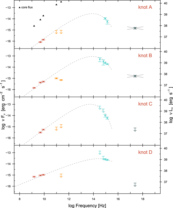
Figure 4. Radio through X-ray fluxes for knots A–D of M84. In the top panel, we also plot the radio fluxes of the core of the jet as black triangles for comparison (note that the ALMA fluxes show no turnover, unlike the ALMA points for knot B). Upper limits are shown as arrows. The gray dashed lines are phenomenological fits to the radio and optical data to show how anomalous the ALMA data points are if we assume a single radio–optical synchrotron spectrum.
Download figure:
Standard image High-resolution image
Table 3. Properties and Multiwavelength Fluxes for the Knots of M84
| Property | Observatory | Frequency (GHz) | Flux Unit | Knot A | Knot B | Knot C | Knot D |
|---|---|---|---|---|---|---|---|
| Distance (kpc) | 0.22 | 0.30 | 0.40 | 0.52 | |||
| Size (pc) | 43 | 50 | 39 | 140 | |||
| FL | VLA | 1.51 × 10⁹ | mJy | … | 9.42 | … | 47 |
| FC | VLA | 4.86 × 10⁹ | mJy | 1.69 | 8.80 | 6.26 | 19.3 |
| FX | VLA | 8.46 × 10⁹ | mJy | 1.60 | 6.02 | 6.50 | 12.5 |
| FB3 | ALMA | 9.75 × 10¹⁰ | mJy | <0.95 | 1.03 | <0.95 | … |
| FB6 | ALMA | 2.36 × 10¹¹ | mJy | <0.4 | 0.30 | <0.66 | <0.53 |
| F850LP | HST | 3.33 × 10¹⁴ | μJy | … | 15 ± 6 | <21 | <42 |
| F475W | HST | 6.31 × 10¹⁴ | μJy | … | 4.8 ± 2.4 | <6 | <7.5 |
| F336W | HST | 8.92 × 10¹⁴ | μJy | 1.2 ± 0.2 | 2.7 ± 0.4 | 1.1 ± 0.3 | 2.9 ± 0.4 |
| F225W | HST | 1.33 × 10¹⁵ | μJy | 0.4 ± 0.15 | 1.4 ± 0.12 | 0.45 ± 0.1 | 1.7 ± 0.2 |
| F1keV | Chandra | 2.42 × 10¹⁷ | nJy | 0.60 ± 0.11 | 0.66 ± 0.12 | <0.32 | <0.08 |
Note. Distances from the core and sizes are converted using an angular distance scale of 89 pc arcsec–1. The sizes of the knots have been measured in the 1988 C-band radio image using a Gaussian fit, except for knot C, which was measured by eye due to lack of compactness for the Gaussian fit. No errors are given for radio and ALMA fluxes, as the measured errors are smaller than the ∼5% error assumed for the flux calibration. No flux measurement for knot A is reported for the two longer-wavelength HST filters due to contamination from galaxy residuals.
Download table as: ASCIITypeset image
The authors are not aware of any other published jet spectrum showing a similar turnover in the radio/submillimeter spectrum, though ALMA observations of jets are not yet extensive. However, previous ALMA observations of resolved jets usually show a continuous spectrum between radio and the optical, as in PKS 0637–752 (Meyer et al. 2017) and for several MSC jets in Breiding et al. (2017). Given the observed turnover in M84, it is implied that the optical/UV comes from a second spectral component. In addition, the flatness of the X-rays, and the level, for knots A and B clearly indicate a third high-energy component, which is not a continuation of the optical/UV. We have ruled out reddening of the optical spectrum using a “dust map” image constructed by taking the ratio of the F336W and F850LP images. Clearly, at least three spectral components are indicated by the SEDs.
It is worth noting that the X-ray jet does not show the well-defined knots seen in the radio and UV. This is apparent in the imaging shown in Figure 3, but is more clearly depicted in the contour line plot shown in Figure 5. Here, we plot the radio flux from the 1988 C-band image as a red line in comparison to the X-ray flux over the same contour line, following a path from the core out along the centers of each radio knot. Contours are also shown for the UV imaging as dashed lines. In all cases, we take a “line average” perpendicular to the line running along the jet, extending out 014, 02, and 034 in the radio, UV, and X-ray (approximately according to the PSF size) in order to yield a smoother contour line (the UV and X-ray images were also smoothed with a 3 × 3 Gaussian kernel). The individual knots are not well-distinguished in the X-ray contour, though there is a strong drop in the flux level after knot B (around 4″), which seems roughly coincident with that in the radio and optical, taking into account the larger PSF of Chandra. The X-ray dominance (ratio of X-ray to radio flux) is clearly highest at the upstream end of the jet, which is similar to many of the powerful MSC quasar jets, such as 3C 273 (Marshall et al. 2001; Jester et al. 2006) and PKS 0827+243 (Jorstad & Marscher 2006).
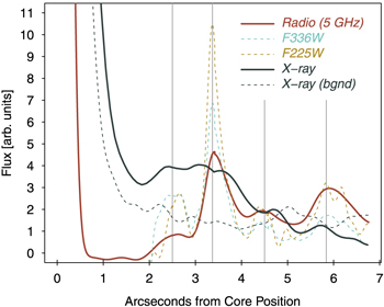
Figure 5. The 5 GHz radio, F225W and F336W HST UV, and Chandra X-ray contour lines following the midline of the jet through the knot centers, as defined by the 5 GHz radio image. Flux units are arbitrary. We show an additional contour line taken from the X-ray image (dashed gray line) from the core through the center of the background region to show that the X-ray level is essentially that of the background by ∼15 from the core. In the jet X-ray contour, some contribution from the inner jet (interior to knot A) contributes to making the core seem to have a larger “wing.”
Download figure:
Standard image High-resolution image
3.2. Optical and Radio Polarization
We examined the total linear polarization image from the ACS/HRC imaging and found no hint of the jet features, with a 3σ upper limit on the polarization percentage of <8% in the area of the jet. However, the fractional polarization in the radio is not as low. In the 1988 C-band image, shown in Figure 6, linear polarization is detected throughout the jet. Around the area of knot B, the highest polarization appears offset to the west but reaches values on the order of 25%, with similar levels in knot D, though somewhat lower in knots A and C (∼10%).
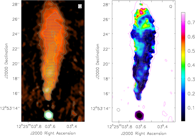
Figure 6. Total intensity C-band (1988) image of the main M84 jet (left panel) and the fractional linear polarization of the same (right panel; intensity scales show fractional polarization level). Overlaid on both are total intensity contours in magenta starting at 0.1 mJy (spaced by factors of 2), and the magnetic field direction as black (white) lines. The data used to create this figure are available.
Download figure:
Standard image High-resolution image
The low polarization in the optical is not necessarily unusual in the context of a synchrotron model (especially given the rather high upper limit), since synchrotron emission can still be produced in an environment with a “tangled” magnetic field which produces linear polarization that effectively cancels out. However, it is somewhat unusual to find that a jet with reasonably high radio polarization lacks polarization in the optical (see, e.g., Perlman et al. 1999, 2006). Deeper optical polarization observations are necessary to get more stringent limits on the optical polarization degree, before any strong conclusions can be drawn about the nature of the optical emission.
3.3. Counterjet Detection and Ratios
We used the lower-resolution imaging in bands L, C, X, and Ku (described in Section 2.3) in order to characterize the jet-to-counterjet ratio. Assuming that the jets are oriented 180 degrees from each other and have a consistent beaming pattern and intrinsic power, this ratio contains information about the speed of the jet and orientation to the line of sight. In particular, the ratio of the jet-to-counterjet flux can be expressed as

where β is the speed of the jet in units of c, θ is the angle of the jet to the line of sight, α is the radio spectral index, and the index m depends on the flow (in the case of moving knots, m = 3 and for a continuous flow m = 2). For M84, we take α = 0.7 and m = 3.
To measure R, we used a contour line at 0.2 mJy around the north and south jets from the U-band image, which yields similarly sized smooth regions surrounding the brightest part of each jet, as shown at left in Figure 7. The purpose of making the measurement at different frequencies was to look for evidence of a change in the ratio with frequency, which might indicate a difference in beaming. However, we did not find such a trend, with values of 1.4, 1.6, 1.2, and 1.3 at the L, C, X and Ku bands, respectively. We thus take the mean value of 1.4 ± 0.2 as representative of the radio R value. Note that the errors on the flux measurement within the contour are very small, less than 1%, though some unaccounted error comes from the exact choice of contour. We verified with several trials that areas of both larger and smaller extent yield similar ratios to the above.
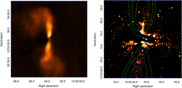
Figure 7. At left, the Ku-band D-configuration image of M84, with a contour line at 0.2 mJy overlaid (the core has been subtracted). The jet (upper) and counterjet (lower) regions were used to measure the jet-to-counterjet flux ratio R. At right, the WFC3/UVIS F336W image after galaxy subtraction and with appropriate scaling to show the faint counterjet. The overlaid contours are from the Ku-band, D-configuration image, at levels of 0.1, 0.2, and 0.4 mJy. The magenta polygon region was used to measure the total flux of the feature. The data used to create this figure are available.
Download figure:
Standard image High-resolution image
3.4. Detection of the UV Counterjet
In addition to the easily seen radio counterjet, we have also detected the counterjet in our the F225W and F336W WFC3/UVIS imaging. This is shown at right in Figure 7 for the F336 image, where contours from the Ku-band/D-configuration image are overlaid. The faint overdensity inside the magenta polygon region has a total flux of 4.8 μJy in the F336W image, after taking into account the slight oversubtraction of the background in the vicinity. The standard deviation of the background level is 0.95 μJy, making this an approximately 5σ detection. Similarly, in the F225W image, using an identically sized and similarly placed region, we measure a flux of 2.1 μJy compared to the background standard deviation of 0.4 μJy, again yielding an approximately 5σ detection. Using a region of comparable size on the main jet, we measure fluxes of 12.3 ± 1.6 and 4.8 ± 0.5 μJy for the F336W and F225W images, respectively. The R value in the UV is thus consistently higher than in the radio at 2.6 ± 0.6 and 2.3 ± 0.5, respectively. This could be explained if the optical/UV is more beamed than the radio, due to a spine/sheath structure in the jet. Such a structure is consistent with the slightly smaller size of the knots in the UV compared to the radio: a factor of 38% for knot D and 30% for knot B, where we used the Gaussian fit tool in casaviewer and average the results for the two UV images (knots A and C did not give reliable Gaussian fits in the UV images).
3.5. Constraints from Proper Motions and the Counterjet
The results of the WISE proper motion analysis yielded a speed of 3.9 ± 1.5 and 3.3 ± 2.5 mas yr−1 for knots A and B, respectively. Results were consistent over a range of pixel scales from 8 to 16, though the errors are relatively large. Taking the knot A measurement as the more constraining, this is equivalent to an apparent speed βapp of 1.1 ± 0.4 c.
Combining the proper motion measurement with the radio jet-to-counterjet ratio yields a single value for the intrinsic speed of the jet as well as the orientation angle. This is shown in Figure 8. Clearly, the data are consistent with M84 having a relatively large angle to the line of sight. Using the bounds reported above on βapp and R, the resulting angle is  °, where the lower bound is found from the maximum R and minimum βapp, and the upper bound from the lower limit of R when the true jet speed is 1, as shown in Figure 8. It is also interesting that the low value of R precludes a value of βapp that is much larger than what we have observed. The angle of 74° corresponds to a β value of 0.87 and a Lorentz factor Γ = 2 (the lower angle limit corresponds to Γ = 1.2).
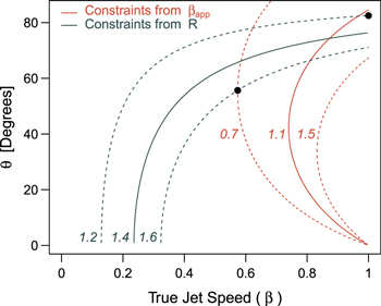
Figure 8. Constraints in the θ–β plane based on the jet-to-counterjet ratio R = 1.4 ± 0.2 (dark gray lines) and proper motions βapp = 1.1 ± 0.4 (orange lines). The resulting best-fit angle to the line of sight is  °. The combination of limits leading to the lower and upper bounds on the angle are noted with black points.
Download figure:
Standard image High-resolution image
4.1. Star Formation
One possibility for optical/UV emission in the vicinity of a relativistic jet is the presence of vigorous star formation induced by the jet impacting dense molecular clouds. Such an origin would be consistent with the lack of optical polarization observed in M84. Direct observation of jet-induced star formation is rare, but it has been observed in a few low-redshift radio galaxies such as Centaurus A (Mould et al. 2000; Salomé et al. 2017), 3C 285 (Salomé et al. 2015), and Minkowski’s Object (van Breugel et al. 1985; Lacy et al. 2017). At higher redshifts, some radio galaxies show an alignment of optical emission with the radio jet axis, which has also been taken as evidence for jet-induced star formation (e.g., McCarthy et al. 1987). However, M84 would be a highly unusual case in comparison with previous cases, since we find that the UV knots perfectly correspond to the radio in location and are actually somewhat more compact. This is similar to what has been found in other jets where there is no ambiguity as to the optical emission being synchrotron, due to spectral continuity and the large distance from the host galaxy (e.g., PKS 0637–752; Meyer et al. 2017). In contrast, previous cases of confirmed jet-induced star formation typically show filamentary structures (as in Centaurus A) or blobs which are displaced from the main radio emission, tending either to lie alongside or toward the jet terminus, and often having much larger angular extent, as in the high-redshift source 4C 41.17 (Bicknell et al. 2000). In these other cases, typical star formation rates are on the order of 1–100 M⊙ yr−1. Using the basic scaling SFRUV = 1.4 × 10⁻²⁸ LUV (Rosa-González et al. 2002) with the far-UV luminosity of knot B (LB = 6 × 10²³ erg s−1 Hz−1), we find that a star formation rate of ∼10−4 M⊙ yr−1 would be implied before accounting for dust reddening, which might make this value 5–10 times higher. This is clearly still too low to be plausible when compared with the dynamical timescale of the jet—knot B, for example, has taken approximately 3 × 10⁴ yr to arrive at its current location. Identical arguments would rule out star formation in the other knots as well, given their similar placement, size, and luminosity. For these reasons, we do not support star formation as a likely origin for the optical/UV emission in the M84 jet.
4.2. Leptonic Models
4.2.1. Inverse Compton Models
If we discount the low ALMA fluxes, a continuous synchrotron spectrum can be fit to the radio–optical data, as shown with a dashed line in Figures 4 and 9. Clearly, given the observed ALMA fluxes and upper limits, these SEDs are not possible. However, even assuming the single radio–optical spectrum were correct, the X-rays are still clearly difficult to account for, being too hard for the falling part of the synchrotron spectrum. As shown in Figure 9 for knot B, an IC/CMB model can be made to fit the X-ray flux level (thick dashed gray line), but again the X-ray spectral index is off, only this time being far too soft, and the model predicts a grossly unrealistic (and ruled out) level of gamma-ray emission, even with a turnover in the synchrotron spectrum at ∼1011 Hz. Finally, the large angle and slow bulk motion implied by the proper motions and counterjet measurements would require the IC/CMB jet to be grossly out of equipartition.
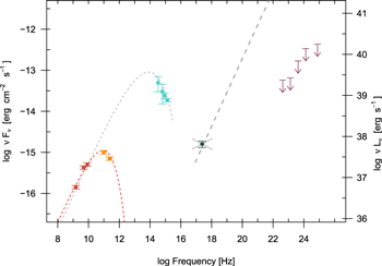
Figure 9. The SED of knot B, along with gamma-ray upper limits from Fermi. The light dashed gray line fits the radio–optical spectrum (ignoring the ALMA data), while the red-dashed line fits the radio and ALMA data only. The X-rays are clearly too high and too hard to be connected to the optical component; however, the spectral index is too soft for an IC/CMB model (thick dashed line at right). Further, an IC/CMB model would overpredict the Fermi limits and require a magnetic field out of equipartition by three orders of magnitude. Only one IC/CMB curve is shown since they are virtually indistinguishable for either of the two synchrotron spectra shown over the range of frequency and flux shown here. Both severely violate all of the Fermi upper limits.
Download figure:
Standard image High-resolution image
Harris et al. (2002) were the first to investigate in depth the possible emission mechanisms for the X-rays from the M84 jet, though without the benefit of the deeper follow-up observations taken in 2005. In that paper, the IC/CMB model is found to be unrealistic along the same lines we find here, and SSC is also ruled out as the photon density in the knot is so low that the predicted 1 keV fluxes are four orders of magnitude below the observed values, assuming equipartition magnetic field strength. Allowing deviations from equipartition to match the observed X-ray fluxes would require a total jet power orders of magnitude larger than the Eddington luminosity and would be unable to produce the flat spectrum in the X-rays—thus, SSC can be ruled out.
4.2.2. Bremsstrahlung Model
Harris et al. (2002) also considered the possibility of thermal bremsstrahlung from relatively dense (5 cm−3) hot gas, but favor a synchrotron interpretation due to the implied high pressure in the emitting region (far higher than the ambient medium), as well as the high temperature (>15 keV) of the gas required under even adiabatic compression of the gas, which does not fit the observations. We confirm that though the best-fit thermal bremsstrahlung model to the X-ray spectrum gives an acceptable fit (reduced-χ2 of 0.65) to the data, the temperature (2.2 ± 0.8 keV) is too low.
4.2.3. Two-component Synchrotron Model
The problems of the inverse Compton models discussed in the previous section lead to the suggestion that the X-rays are also produced via synchrotron radiation from a second electron population residing in the knot (e.g., Hardcastle 2006; Uchiyama et al. 2006; Kataoka et al. 2008).
In this scenario, the radio and ALMA data are attributed to the synchrotron emission of the first electron population ( ), while the second electron population (
 ) is responsible for the optical-to-X-ray emission of the knot. The different photon indices in the optical/UV and X-ray energy bands suggest that the underlying electron distribution is more complicated than a single power law. This could be a broken power law, although the hardening of the distribution above the break cannot be easily explained. Another possibility, which we adopt here, is that of a relativistic Maxwellian with “temperature” γth ≫ 1 (in units of mec2), smoothly connected to a power law from γnth > γth (e.g., Giannios & Spitkovsky 2009). The particle distribution at injection can be written as
We assume that both electron distributions are described by Equation (2), although the radio and ALMA data can be explained by a single power-law electron distribution. All of the model parameters of  can be constrained by the data, except for the maximum Lorentz factor, whereas all the power-law parameters of
  remain unconstrained. These were assumed to be the same as those of the second electron population in order to reduce the number of free parameters. Moreover, we searched for parameter sets that result in (rough) energy equipartition between the magnetic field and the particles in the knot.
Using the one-zone time-dependent numerical code of Dimitrakoudis et al. (2012), we computed the steady-state photon and particle spectra within the two-component synchrotron scenario. Our fitting results are presented in Figure 10, and the parameter values are summarized in Table 4. For these parameter values, we find that uB = 4 × 10⁻¹⁰ erg cm−3,  erg cm−3, and that the power of a one-sided jet is ∼6 × 1042 erg s−1.
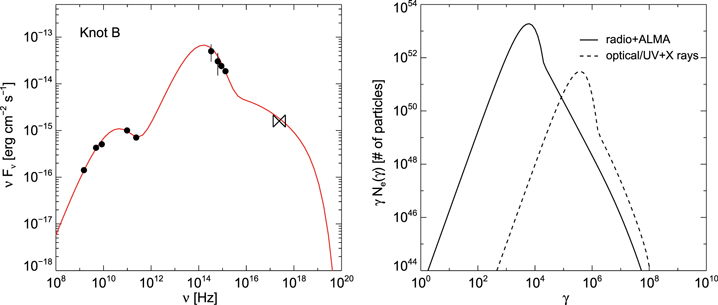
Figure 10. Left panel: two-component synchrotron fit (red solid line) to the SED of knot B (black symbols). Right panel: steady-state electron distributions invoked to explain the SED of knot B (right panel). We assumed that both can be described by a relativistic Maxwellian distribution with a power law. We find rough energy equipartition between the magnetic field and particles in knot B.
Download figure:
Standard image High-resolution image
Table 4. Parameters of the Two-component Synchrotron Model Presented in Figure 10
| Symbol | Parameter | Value | |
|---|---|---|---|
| B [mG] | Magnetic field strength | 0.1 | |
| R [pc] | Knot size | 50 | |
| δ | Doppler factor | 1 | |

|

|
||
| Le [erg s−1] | Injection luminosity | 8.8 × 1041 | 8.8 × 1041 |
| γth [mec2] | “Temperature” of Maxwellian | 2 × 10³ | 1.3 × 10⁵ |
| γnth | Min. Lorentz factor of power law | 2 × 10⁴ | 1.3 × 10⁶ |
| γmax | Max. Lorentz factor of power law | 108 | 108 |
| s | Power-law index | 3 | 3 |
Download table as: ASCIITypeset image
Despite the success of the model in reproducing the multicomponent SED for equipartition conditions in the knot, it relies on the ad hoc assumption of two electron populations. There is no good explanation for the generation of relativistic Maxwellian distributions with temperatures that differ by almost four orders of magnitude, in a flow that is barely relativistic (see Sections 3.3 and 3.4).
4.3. Leptohadronic Model
Models that consider the radiation produced by relativistic electrons and protons, the so-called leptohadronic models, pose an interesting alternative to the pure leptonic scenarios discussed in the previous section, as they can naturally produce multicomponent SEDs (for blazars, see, e.g., Petropoulou et al. 2015, 2017; for large-scale jets, see, e.g., Aharonian 2002, Bhattacharyya & Gupta 2016, and Kusunose & Takahara 2017). Here, we focus on the SED of the brightest and, thus, best-sampled knot of the jet (knot B).
We model knot B10
as a spherical blob of radius R = 50 pc containing a tangled magnetic field of strength B. Protons and electrons are assumed to be accelerated to relativistic energies and to be subsequently injected isotropically into the volume of the blob at a constant rate. Particles are also assumed to escape from the knot on a characteristic timescale of R/c. The accelerated particle distributions at injection are modeled as power laws between a minimum (γi,min) and a maximum (γi,max) Lorentz factor, namely  where i = e, p stands for electrons and protons.
At any time, the relativistic electron population is comprised of those that have undergone acceleration (primaries) and those that have been produced by other processes (secondaries). These include (i) the direct production through the Bethe–Heitler (BH) process  , (ii) the decay of π± produced via the photopion process, i.e.,
  ,
,  , and (iii) the photon–photon absorption
  . Secondary electrons also radiate via synchrotron and inverse Compton scattering processes. Due to the different energy distributions of the primary and secondary electrons, the resulting SED will be, in general, comprised of multiple components.
4.3.1. Analytical Estimates
The SED of knot B shows at least three components: the first (C1) peaks at ν1 ≃ 100 GHz with a peak luminosity L1,pk ≃ 4 × 1037 erg s−1, the second (C2) extends from submillimeter to UV wavelengths with a likely peak at ν2 ≃ 1014 Hz and luminosity L2,pk ≃ 3 × 1039 erg s−1, and the third (C3) emerges in the X-ray energy band.
Components C1 and C2 can be naturally explained as the synchrotron radiation of primary electrons and protons, respectively. In a magnetic field B = 1 BmG mG, the typical Lorentz factor of electrons and protons radiating at ν1 and ν2, respectively, is  and
and  . The spectral shapes of the two components also suggest that se ∼ 2, γe,max ≃ γe,pk, sp ∼ 4, and γp,min ≃ γp,pk. Moreover, the maximum proton Lorentz factor cannot be arbitrarily large, as the synchrotron spectrum would extend to the X-rays, yielding a much softer spectral index than observed. Thus, γp,max ≲ 10γp,pk.
Protons with  may directly produce secondary electrons with a wide range of Lorentz factors, i.e., from
  to
to  where we used γp,max = 10γp,pk. Their distribution can be approximated by a power law with slope p ≃ sp, while their synchrotron emission may emerge in the X-rays. The synchrotron spectrum can be approximately modeled as

where β = (p − 1)/2, νmin ∼ 1015 Hz, νmax ∼ 1023 Hz, Lp is the proton luminosity, and fBH is a measure of the photopair production efficiency. This is defined as fBH ≡ R σBH n2, where σBH ≈ 10−27 cm2 is the average cross-section, and n2 ≃ 3L2,pk/4πR2chν2. Due to the very low number density of target photons, photopair production is inefficient:

The observed X-ray luminosity, LX ≃ 8 × 1037 erg s−1, can be thus explained by synchrotron emission of BH electrons (Equation (3)), if the proton luminosity is sufficiently high, namely

The synchrotron emission from secondary electrons produced in photopion interactions is expected to extend to even higher energies and be less luminous than the synchrotron radiation of BH pairs (see also Kusunose & Takahara 2017).
4.3.2. Numerical Modeling
Here, we expand upon the scenario outlined in the previous section by performing detailed numerical calculations of the SED. For this purpose, we use the one-zone time-dependent leptohadronic numerical code of Dimitrakoudis et al. (2012), which includes all relevant radiative processes with the full expressions for the cross-sections and injection rates of secondaries.
We search for the best-fit parameter values by using as a starting point the rough estimates presented in the previous section. We consider as targets for photohadronic interactions only the photons produced in knot B. We obtain the steady-state photon spectra after running the code for 610 light-crossing times of the knot or 105 yr. Our best-fit parameter values are summarized in Table 5 and the resulting spectra are presented in Figure 11. The multicomponent SED of knot B can be successfully described within the leptohadronic scenario. Because of the low number density of photons that are targets for photohadronic interactions, the proton luminosity must be about 10 times larger than the Eddington luminosity of the source to explain the X-ray flux of knot B (Table 5).
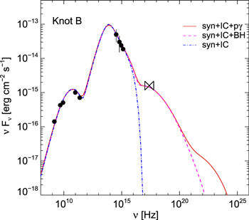
Figure 11. Leptohadronic fit (red solid line) to the SED of knot B (black symbols) where the radio peak is attributed to synchrotron radiation from electrons, the optical peak to synchrotron radiation from protons, and the X-rays are attributed to the synchrotron radiation of secondary electrons from the Bethe–Heitler process. Overplotted (magenta dashed line) is the spectrum computed without photopion interactions (inverse Compton emission is included in the model although it is negligible here). The contribution of Bethe–Heitler pairs in X-rays is now evident. The spectrum obtained in the absence of photopion and photopair interactions is also shown for comparison (blue dashed–dotted line). The model parameters are summarized in Table 5.
Download figure:
Standard image High-resolution image
Table 5. Parameters of the Leptohadronic Model Presented in Figure 11
| Symbol | Parameter | Value |
|---|---|---|
| B [mG] | Magnetic field strength | 1 |
| R [pc] | Knot size | 50 |
| δ | Doppler factor | 1 |
| Le [erg s−1] | Electron luminosity (primary) | 9 × 1039 |
| γe,min | Min. electron Lorentz factor | 103 |
| γe,max | Max. electron Lorentz factor | 5 × 10³ |
| se | Electron power-law index | 2 |
| Lp [erg s−1] | Proton luminosity | 2 × 1048a |
| γp,min | Min. proton Lorentz factor | 3 × 10⁶ |
| γp,max | Max. proton Lorentz factor | 5 × 10⁷ |
| sp | Proton power-law index | 4.4 |
Note.
aThe best-fit value of Lp is 10 times larger than the rough estimate (Equation (5)) due to the simplifying assumptions entering the analytical calculation.Download table as: ASCIITypeset image
The energetic requirements could relax, if there were external optical photons with a higher energy density than those produced internally in the knot. More specifically, the required proton luminosity could be reduced to 1046 erg s−1, only if the energy density of optical photons was ∼10−9 erg cm−3. Yet, the density of optical photons from both the core and the galaxy itself is many orders of magnitudes lower.
It is difficult at present to distinguish between the leptonic and hadronic scenarios with present capabilities. However, high-resolution imaging in the hard X-rays, with sufficient statistics to determine the hard X-ray spectrum of the knots, could help distinguish and inform jet models. Given the upper limit on the optical polarization, future high-resolution X-ray polarization imaging of the knots would be useful to check the assumption of co-spatiality.
In this paper, we report the detection of a resolved optical/UV jet in M84, extending ∼0.5 kpc from the core, as well as a counterjet detected at 5σ in near- and far-UV HST imaging. Combining archival VLA, ALMA, HST, and Chandra imaging of the jet in M84, we have constructed a well-sampled SED for the kiloparsec-scale jet in M84 for the first time. We find evidence for a spectral turnover at ∼100 GHz, which has not been previously observed in any large-scale jet. Along with the high optical flux and relatively hard X-ray emission, this implies at least three distinct spectral components in the M84 jet. Archival HST polarization imaging in the F606W band finds no optical polarization in the jet, with an upper limit on the fractional linear polarization of 8%. In contrast, the radio jet shows typical linear polarization fractions of 10%–30%. We rule out star formation as the origin of the optical/UV emission based on the low UV luminosity. Leptonic inverse Compton models are ruled out on the basis of requiring extreme departures from equipartition and predicting a high gamma-ray flux, which is not observed. We have explored the possibility of a dual population of relativistic electrons with relativistic Maxwellian distributions, coupled with a power-law extension at high energies. While such a model can fit the observed SED of knot B in the jet, the model is ad hoc, and there is no explanation of the extreme temperature difference between the components. We also explore a leptohadronic model in which the radio and optical emission can be attributed to synchrotron emission from relativistic electrons and protons, respectively, while the X-rays are due to synchrotron emission from electron secondaries. However, such a model requires a total power in relativistic protons that is 10 times the Eddington limit. At present, we lack a comprehensive understanding of the physics of the emitting regions in the M84 jet. These unusual features are not predicted by any known model of jet emission.
E.T.M. and M.G. acknowledge NASA ADAP grant NNX15AE55G and NASA Fermi grant NNX15AU78G. M.P. acknowledges support by the L. Spitzer Postdoctoral Fellowship. M.P. would like to thank Dr. Dimitrakoudis and Prof. Mastichiadis for providing the numerical code. This paper makes use of the following ALMA data: ADS/JAO.ALMA#2013.1.00828.S and ADS/JAO.ALMA#2015.1.01170.S. ALMA is a partnership of ESO (representing its member states), NSF (USA) and NINS (Japan), together with NRC (Canada), MOST and ASIAA (Taiwan), and KASI (Republic of Korea), in cooperation with the Republic of Chile. The Joint ALMA Observatory is operated by ESO, AUI/NRAO, and NAOJ.
Facilities: VLA - Very Large Array, ALMA - , HST - , Chandra - , Fermi - .
Software: CASA, IDL, IRAF, CIAO, astropy.