Choose univariate class intervals — classIntervals
if (!require("spData", quietly=TRUE)) {
message("spData package needed for examples")
run <- FALSE
} else {
run <- TRUE
}
if (run) {
data(jenks71, package="spData")
pal1 <- c("wheat1", "red3")
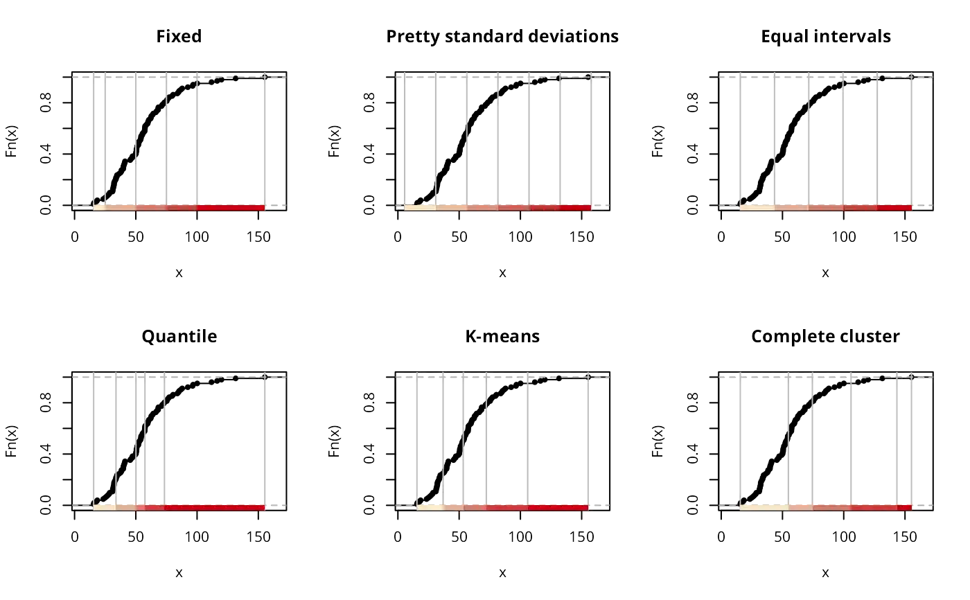
opar <- par(mfrow=c(2,3))
plot(classIntervals(jenks71$jenks71, n=5, style="fixed",
fixedBreaks=c(15.57, 25, 50, 75, 100, 155.30)), pal=pal1, main="Fixed")
plot(classIntervals(jenks71$jenks71, n=5, style="sd"), pal=pal1, main="Pretty standard deviations")
plot(classIntervals(jenks71$jenks71, n=5, style="equal"), pal=pal1, main="Equal intervals")
plot(classIntervals(jenks71$jenks71, n=5, style="quantile"), pal=pal1, main="Quantile")
set.seed(1)
plot(classIntervals(jenks71$jenks71, n=5, style="kmeans"), pal=pal1, main="K-means")
plot(classIntervals(jenks71$jenks71, n=5, style="hclust", method="complete"),
pal=pal1, main="Complete cluster")
}
 if (run) {
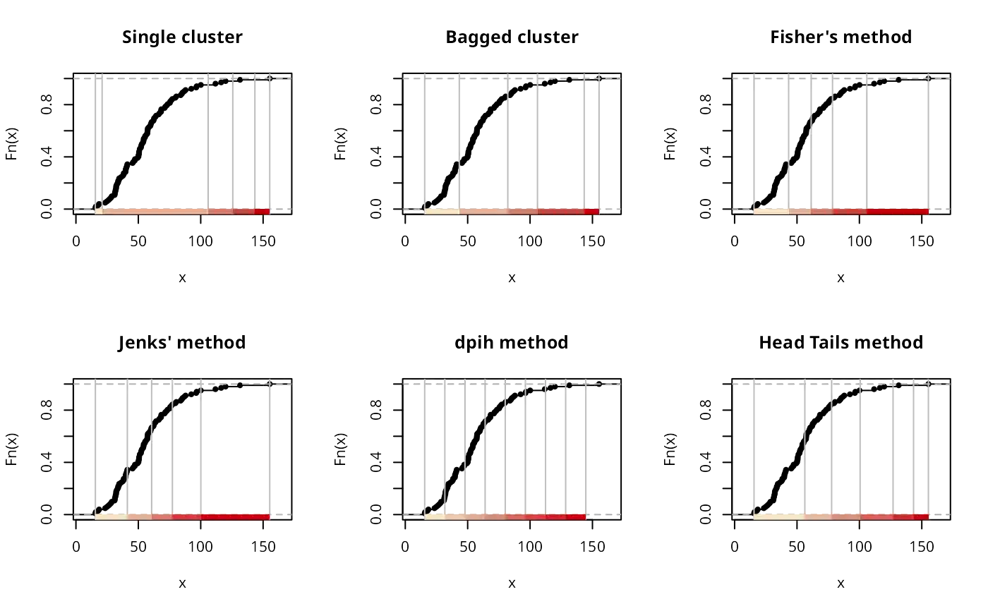
plot(classIntervals(jenks71$jenks71, n=5, style="hclust", method="single"),
pal=pal1, main="Single cluster")
set.seed(1)
plot(classIntervals(jenks71$jenks71, n=5, style="bclust", verbose=FALSE),
pal=pal1, main="Bagged cluster")
plot(classIntervals(jenks71$jenks71, n=5, style="fisher"), pal=pal1,
main="Fisher's method")
plot(classIntervals(jenks71$jenks71, n=5, style="jenks"), pal=pal1,
main="Jenks' method")
plot(classIntervals(jenks71$jenks71, style="dpih"), pal=pal1,
main="dpih method")
plot(classIntervals(jenks71$jenks71, style="headtails", thr = 1), pal=pal1,
main="Head Tails method")
}
if (run) {
plot(classIntervals(jenks71$jenks71, n=5, style="hclust", method="single"),
pal=pal1, main="Single cluster")
set.seed(1)
plot(classIntervals(jenks71$jenks71, n=5, style="bclust", verbose=FALSE),
pal=pal1, main="Bagged cluster")
plot(classIntervals(jenks71$jenks71, n=5, style="fisher"), pal=pal1,
main="Fisher's method")
plot(classIntervals(jenks71$jenks71, n=5, style="jenks"), pal=pal1,
main="Jenks' method")
plot(classIntervals(jenks71$jenks71, style="dpih"), pal=pal1,
main="dpih method")
plot(classIntervals(jenks71$jenks71, style="headtails", thr = 1), pal=pal1,
main="Head Tails method")
}
 if (run) {
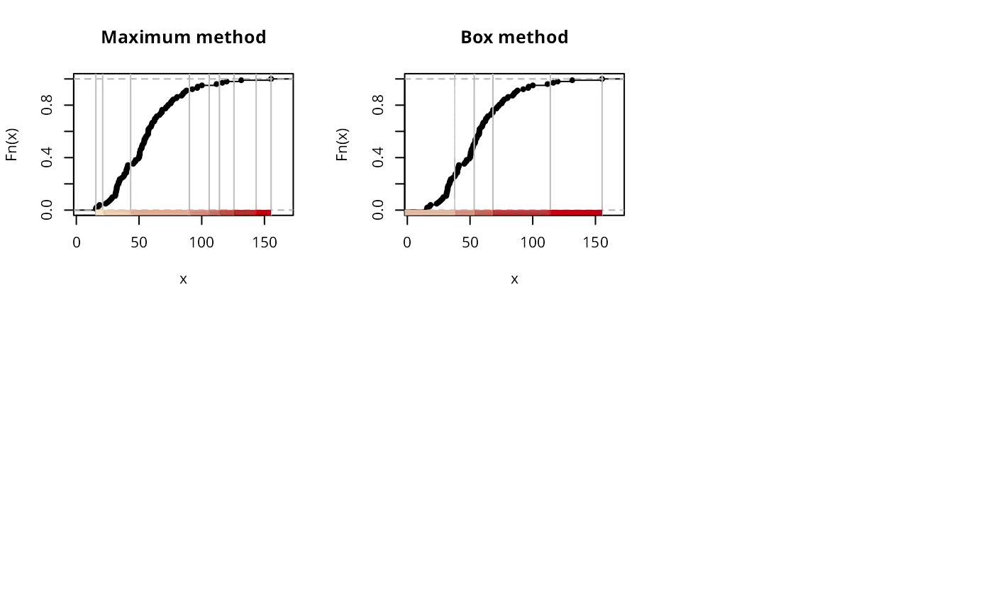
plot(classIntervals(jenks71$jenks71, style="maximum"), pal=pal1,
main="Maximum method")
plot(classIntervals(jenks71$jenks71, style="box"), pal=pal1,
main="Box method")
par(opar)
}
if (run) {
plot(classIntervals(jenks71$jenks71, style="maximum"), pal=pal1,
main="Maximum method")
plot(classIntervals(jenks71$jenks71, style="box"), pal=pal1,
main="Box method")
par(opar)
}
 if (run) {
print(classIntervals(jenks71$jenks71, n=5, style="fixed",
fixedBreaks=c(15.57, 25, 50, 75, 100, 155.30)))
}
#> style: fixed
#> one of 3,921,225 possible partitions of this variable into 5 classes
#> [15.57,25) [25,50) [50,75) [75,100) [100,155.3]
#> 6 34 42 14 6
if (run) {
print(classIntervals(jenks71$jenks71, n=5, style="sd"))
}
#> style: sd
#> one of 75,287,520 possible partitions of this variable into 6 classes
#> [5.514407,30.89691) [30.89691,56.27941) [56.27941,81.66191) [81.66191,107.0444)
#> 10 47 31 9
#> [107.0444,132.4269) [132.4269,157.8094]
#> 4 1
if (run) {
print(classIntervals(jenks71$jenks71, n=5, style="equal"))
}
#> style: equal
#> one of 3,921,225 possible partitions of this variable into 5 classes
#> [15.57,43.516) [43.516,71.462) [71.462,99.408) [99.408,127.354)
#> 35 44 17 4
#> [127.354,155.3]
#> 2
if (run) {
print(classIntervals(jenks71$jenks71, n=5, style="quantile"))
}
#> style: quantile
#> one of 3,921,225 possible partitions of this variable into 5 classes
#> [15.57,33.822) [33.822,50.114) [50.114,57.454) [57.454,73.368) [73.368,155.3]
#> 21 20 20 20 21
if (run) {
set.seed(1)
print(classIntervals(jenks71$jenks71, n=5, style="kmeans"))
}
#> style: kmeans
#> one of 3,921,225 possible partitions of this variable into 5 classes
#> [15.57,36.905) [36.905,53.33) [53.33,72.185) [72.185,105.95) [105.95,155.3]
#> 25 26 29 17 5
if (run) {
set.seed(1)
print(classIntervals(jenks71$jenks71, n=5, style="kmeans", intervalClosure="right"))
}
#> style: kmeans
#> one of 3,921,225 possible partitions of this variable into 5 classes
#> [15.57,36.905] (36.905,53.33] (53.33,72.185] (72.185,105.95] (105.95,155.3]
#> 25 26 29 17 5
if (run) {
set.seed(1)
print(classIntervals(jenks71$jenks71, n=5, style="kmeans", dataPrecision=0))
}
#> style: kmeans
#> one of 3,921,225 possible partitions of this variable into 5 classes
#> [16,37) [37,54) [54,73) [73,106) [106,156]
#> 25 26 29 17 5
if (run) {
set.seed(1)
print(classIntervals(jenks71$jenks71, n=5, style="kmeans"), cutlabels=FALSE)
}
#> style: kmeans
#> one of 3,921,225 possible partitions of this variable into 5 classes
#> under 36.905 36.905 - 53.33 53.33 - 72.185 72.185 - 105.95 over 105.95
#> 25 26 29 17 5
if (run) {
print(classIntervals(jenks71$jenks71, n=5, style="hclust", method="complete"))
}
#> style: hclust
#> one of 3,921,225 possible partitions of this variable into 5 classes
#> [15.57,54.81) [54.81,74.405) [74.405,105.95) [105.95,143.4) [143.4,155.3]
#> 55 27 15 4 1
if (run) {
print(classIntervals(jenks71$jenks71, n=5, style="hclust", method="single"))
}
#> style: hclust
#> one of 3,921,225 possible partitions of this variable into 5 classes
#> [15.57,20.995) [20.995,105.95) [105.95,125.7) [125.7,143.4) [143.4,155.3]
#> 4 93 3 1 1
if (run) {
set.seed(1)
print(classIntervals(jenks71$jenks71, n=5, style="bclust", verbose=FALSE))
}
#> style: bclust
#> one of 3,921,225 possible partitions of this variable into 5 classes
#> [15.57,43.3) [43.3,82.175) [82.175,105.95) [105.95,143.4) [143.4,155.3]
#> 35 53 9 4 1
if (run) {
print(classIntervals(jenks71$jenks71, n=5, style="bclust",
hclust.method="complete", verbose=FALSE))
}
#> style: bclust
#> one of 3,921,225 possible partitions of this variable into 5 classes
#> [15.57,43.3) [43.3,82.175) [82.175,105.95) [105.95,143.4) [143.4,155.3]
#> 35 53 9 4 1
if (run) {
print(classIntervals(jenks71$jenks71, n=5, style="fisher"))
}
#> style: fisher
#> one of 3,921,225 possible partitions of this variable into 5 classes
#> [15.57,43.3) [43.3,61.36) [61.36,78.475) [78.475,105.95) [105.95,155.3]
#> 35 33 18 11 5
if (run) {
print(classIntervals(jenks71$jenks71, n=5, style="jenks"))
}
#> style: jenks
#> one of 3,921,225 possible partitions of this variable into 5 classes
#> [15.57,41.2] (41.2,60.66] (60.66,77.29] (77.29,100.1] (100.1,155.3]
#> 35 33 18 11 5
if (run) {
print(classIntervals(jenks71$jenks71, style="dpih"))
}
#> style: dpih
#> one of 16,007,560,800 possible partitions of this variable into 8 classes
#> [15.57,31.70792) [31.70792,47.84584) [47.84584,63.98376) [63.98376,80.12169)
#> 14 25 33 15
#> [80.12169,96.25961) [96.25961,112.3975) [112.3975,128.5355) [128.5355,144.6734]
#> 7 4 2 2
if (run) {
print(classIntervals(jenks71$jenks71, style="dpih", range.x=c(0, 160)))
}
#> style: dpih
#> one of 186,087,894,300 possible partitions of this variable into 9 classes
#> [0,16.26458) [16.26458,32.52917) [32.52917,48.79375) [48.79375,65.05834)
#> 2 16 21 34
#> [65.05834,81.32292) [81.32292,97.58751) [97.58751,113.8521) [113.8521,130.1167)
#> 15 8 2 2
#> [130.1167,146.3813]
#> 2
if (run) {
print(classIntervals(jenks71$jenks71, style="headtails"))
}
#> style: headtails
#> one of 100 possible partitions of this variable into 2 classes
#> [15.57,56.27941) [56.27941,155.3]
#> 57 45
if (run) {
print(classIntervals(jenks71$jenks71, style="headtails", thr = .45))
}
#> style: headtails
#> one of 75,287,520 possible partitions of this variable into 6 classes
#> [15.57,56.27941) [56.27941,77.74533) [77.74533,100.5925) [100.5925,126.98)
#> 57 29 11 3
#> [126.98,143.4) [143.4,155.3]
#> 1 1
if (run) {
print(classIntervals(jenks71$jenks71, style="maximum"))
}
#> style: maximum
#> one of 16,007,560,800 possible partitions of this variable into 8 classes
#> [15.57,20.995) [20.995,43.3) [43.3,90.16) [90.16,105.95) [105.95,114.1)
#> 4 31 58 4 1
#> [114.1,125.7) [125.7,143.4) [143.4,155.3]
#> 2 1 1
if (run) {
print(classIntervals(jenks71$jenks71, style="box"))
}
#> style: box
#> one of 75,287,520 possible partitions of this variable into 6 classes
#> [-Inf,-8.02125) [-8.02125,37.7325) [37.7325,53.33) [53.33,68.235)
#> 0 26 25 25
#> [68.235,113.9887) [113.9887,155.3]
#> 22 4
if (run) {
print(classIntervals(jenks71$jenks71, style="box", iqr_mult = 0.25))
}
#> style: box
#> one of 75,287,520 possible partitions of this variable into 6 classes
#> [15.57,30.10688) [30.10688,37.7325) [37.7325,53.33) [53.33,68.235)
#> 10 16 25 25
#> [68.235,75.86062) [75.86062,155.3]
#> 8 18
x <- c(0, 0, 0, 1, 2, 50)
print(classIntervals(x, n=3, style="fisher"))
#> style: fisher
#> one of 3 possible partitions of this variable into 3 classes
#> [0,0.5) [0.5,26) [26,50]
#> 3 2 1
print(classIntervals(x, n=3, style="jenks"))
#> style: jenks
#> one of 3 possible partitions of this variable into 3 classes
#> [0,0] (0,2] (2,50]
#> 3 2 1
# Argument 'unique' will collapse the label of classes containing a
# single value. This is particularly useful for 'censored' variables
# that contain for example many zeros.
data_censored<-c(rep(0,10), rnorm(100, mean=20,sd=1),rep(26,10))
plot(density(data_censored))
if (run) {
print(classIntervals(jenks71$jenks71, n=5, style="fixed",
fixedBreaks=c(15.57, 25, 50, 75, 100, 155.30)))
}
#> style: fixed
#> one of 3,921,225 possible partitions of this variable into 5 classes
#> [15.57,25) [25,50) [50,75) [75,100) [100,155.3]
#> 6 34 42 14 6
if (run) {
print(classIntervals(jenks71$jenks71, n=5, style="sd"))
}
#> style: sd
#> one of 75,287,520 possible partitions of this variable into 6 classes
#> [5.514407,30.89691) [30.89691,56.27941) [56.27941,81.66191) [81.66191,107.0444)
#> 10 47 31 9
#> [107.0444,132.4269) [132.4269,157.8094]
#> 4 1
if (run) {
print(classIntervals(jenks71$jenks71, n=5, style="equal"))
}
#> style: equal
#> one of 3,921,225 possible partitions of this variable into 5 classes
#> [15.57,43.516) [43.516,71.462) [71.462,99.408) [99.408,127.354)
#> 35 44 17 4
#> [127.354,155.3]
#> 2
if (run) {
print(classIntervals(jenks71$jenks71, n=5, style="quantile"))
}
#> style: quantile
#> one of 3,921,225 possible partitions of this variable into 5 classes
#> [15.57,33.822) [33.822,50.114) [50.114,57.454) [57.454,73.368) [73.368,155.3]
#> 21 20 20 20 21
if (run) {
set.seed(1)
print(classIntervals(jenks71$jenks71, n=5, style="kmeans"))
}
#> style: kmeans
#> one of 3,921,225 possible partitions of this variable into 5 classes
#> [15.57,36.905) [36.905,53.33) [53.33,72.185) [72.185,105.95) [105.95,155.3]
#> 25 26 29 17 5
if (run) {
set.seed(1)
print(classIntervals(jenks71$jenks71, n=5, style="kmeans", intervalClosure="right"))
}
#> style: kmeans
#> one of 3,921,225 possible partitions of this variable into 5 classes
#> [15.57,36.905] (36.905,53.33] (53.33,72.185] (72.185,105.95] (105.95,155.3]
#> 25 26 29 17 5
if (run) {
set.seed(1)
print(classIntervals(jenks71$jenks71, n=5, style="kmeans", dataPrecision=0))
}
#> style: kmeans
#> one of 3,921,225 possible partitions of this variable into 5 classes
#> [16,37) [37,54) [54,73) [73,106) [106,156]
#> 25 26 29 17 5
if (run) {
set.seed(1)
print(classIntervals(jenks71$jenks71, n=5, style="kmeans"), cutlabels=FALSE)
}
#> style: kmeans
#> one of 3,921,225 possible partitions of this variable into 5 classes
#> under 36.905 36.905 - 53.33 53.33 - 72.185 72.185 - 105.95 over 105.95
#> 25 26 29 17 5
if (run) {
print(classIntervals(jenks71$jenks71, n=5, style="hclust", method="complete"))
}
#> style: hclust
#> one of 3,921,225 possible partitions of this variable into 5 classes
#> [15.57,54.81) [54.81,74.405) [74.405,105.95) [105.95,143.4) [143.4,155.3]
#> 55 27 15 4 1
if (run) {
print(classIntervals(jenks71$jenks71, n=5, style="hclust", method="single"))
}
#> style: hclust
#> one of 3,921,225 possible partitions of this variable into 5 classes
#> [15.57,20.995) [20.995,105.95) [105.95,125.7) [125.7,143.4) [143.4,155.3]
#> 4 93 3 1 1
if (run) {
set.seed(1)
print(classIntervals(jenks71$jenks71, n=5, style="bclust", verbose=FALSE))
}
#> style: bclust
#> one of 3,921,225 possible partitions of this variable into 5 classes
#> [15.57,43.3) [43.3,82.175) [82.175,105.95) [105.95,143.4) [143.4,155.3]
#> 35 53 9 4 1
if (run) {
print(classIntervals(jenks71$jenks71, n=5, style="bclust",
hclust.method="complete", verbose=FALSE))
}
#> style: bclust
#> one of 3,921,225 possible partitions of this variable into 5 classes
#> [15.57,43.3) [43.3,82.175) [82.175,105.95) [105.95,143.4) [143.4,155.3]
#> 35 53 9 4 1
if (run) {
print(classIntervals(jenks71$jenks71, n=5, style="fisher"))
}
#> style: fisher
#> one of 3,921,225 possible partitions of this variable into 5 classes
#> [15.57,43.3) [43.3,61.36) [61.36,78.475) [78.475,105.95) [105.95,155.3]
#> 35 33 18 11 5
if (run) {
print(classIntervals(jenks71$jenks71, n=5, style="jenks"))
}
#> style: jenks
#> one of 3,921,225 possible partitions of this variable into 5 classes
#> [15.57,41.2] (41.2,60.66] (60.66,77.29] (77.29,100.1] (100.1,155.3]
#> 35 33 18 11 5
if (run) {
print(classIntervals(jenks71$jenks71, style="dpih"))
}
#> style: dpih
#> one of 16,007,560,800 possible partitions of this variable into 8 classes
#> [15.57,31.70792) [31.70792,47.84584) [47.84584,63.98376) [63.98376,80.12169)
#> 14 25 33 15
#> [80.12169,96.25961) [96.25961,112.3975) [112.3975,128.5355) [128.5355,144.6734]
#> 7 4 2 2
if (run) {
print(classIntervals(jenks71$jenks71, style="dpih", range.x=c(0, 160)))
}
#> style: dpih
#> one of 186,087,894,300 possible partitions of this variable into 9 classes
#> [0,16.26458) [16.26458,32.52917) [32.52917,48.79375) [48.79375,65.05834)
#> 2 16 21 34
#> [65.05834,81.32292) [81.32292,97.58751) [97.58751,113.8521) [113.8521,130.1167)
#> 15 8 2 2
#> [130.1167,146.3813]
#> 2
if (run) {
print(classIntervals(jenks71$jenks71, style="headtails"))
}
#> style: headtails
#> one of 100 possible partitions of this variable into 2 classes
#> [15.57,56.27941) [56.27941,155.3]
#> 57 45
if (run) {
print(classIntervals(jenks71$jenks71, style="headtails", thr = .45))
}
#> style: headtails
#> one of 75,287,520 possible partitions of this variable into 6 classes
#> [15.57,56.27941) [56.27941,77.74533) [77.74533,100.5925) [100.5925,126.98)
#> 57 29 11 3
#> [126.98,143.4) [143.4,155.3]
#> 1 1
if (run) {
print(classIntervals(jenks71$jenks71, style="maximum"))
}
#> style: maximum
#> one of 16,007,560,800 possible partitions of this variable into 8 classes
#> [15.57,20.995) [20.995,43.3) [43.3,90.16) [90.16,105.95) [105.95,114.1)
#> 4 31 58 4 1
#> [114.1,125.7) [125.7,143.4) [143.4,155.3]
#> 2 1 1
if (run) {
print(classIntervals(jenks71$jenks71, style="box"))
}
#> style: box
#> one of 75,287,520 possible partitions of this variable into 6 classes
#> [-Inf,-8.02125) [-8.02125,37.7325) [37.7325,53.33) [53.33,68.235)
#> 0 26 25 25
#> [68.235,113.9887) [113.9887,155.3]
#> 22 4
if (run) {
print(classIntervals(jenks71$jenks71, style="box", iqr_mult = 0.25))
}
#> style: box
#> one of 75,287,520 possible partitions of this variable into 6 classes
#> [15.57,30.10688) [30.10688,37.7325) [37.7325,53.33) [53.33,68.235)
#> 10 16 25 25
#> [68.235,75.86062) [75.86062,155.3]
#> 8 18
x <- c(0, 0, 0, 1, 2, 50)
print(classIntervals(x, n=3, style="fisher"))
#> style: fisher
#> one of 3 possible partitions of this variable into 3 classes
#> [0,0.5) [0.5,26) [26,50]
#> 3 2 1
print(classIntervals(x, n=3, style="jenks"))
#> style: jenks
#> one of 3 possible partitions of this variable into 3 classes
#> [0,0] (0,2] (2,50]
#> 3 2 1
# Argument 'unique' will collapse the label of classes containing a
# single value. This is particularly useful for 'censored' variables
# that contain for example many zeros.
data_censored<-c(rep(0,10), rnorm(100, mean=20,sd=1),rep(26,10))
plot(density(data_censored))
 cl2 <- classIntervals(data_censored, n=5, style="jenks", dataPrecision=2)
print(cl2, unique=FALSE)
#> style: jenks
#> one of 4,082,925 possible partitions of this variable into 5 classes
#> [0,0] (0,19.5] (19.5,20.63] (20.63,22.6] (22.6,26]
#> 10 33 39 28 10
print(cl2, unique=TRUE)
#> style: jenks
#> one of 4,082,925 possible partitions of this variable into 5 classes
#> Class found with one single (possibly repeated) value: changed label
#> 0 (0,19.5] (19.5,20.63] (20.63,22.6] 26
#> 10 33 39 28 10
# \dontrun{
set.seed(1)
n <- 1e+05
x <- runif(n)
classIntervals(x, n=5, style="sd")
#> style: sd
#> [-0.07925682,0.06546355) [0.06546355,0.2101839) [0.2101839,0.3549043)
#> 6597 14579 14403
#> [0.3549043,0.4996247) [0.4996247,0.644345) [0.644345,0.7890654)
#> 14395 14446 14439
#> [0.7890654,0.9337858) [0.9337858,1.078506]
#> 14463 6678
classIntervals(x, n=5, style="pretty")
#> style: pretty
#> [0,0.2) [0.2,0.4) [0.4,0.6) [0.6,0.8) [0.8,1]
#> 20142 19936 19888 19993 20041
classIntervals(x, n=5, style="equal")
#> style: equal
#> [3.895489e-06,0.1999925) [0.1999925,0.3999812) [0.3999812,0.5999698)
#> 20141 19935 19888
#> [0.5999698,0.7999584) [0.7999584,0.9999471]
#> 19991 20045
classIntervals(x, n=5, style="quantile")
#> style: quantile
#> [3.895489e-06,0.1984408) [0.1984408,0.3993007) [0.3993007,0.6003913)
#> 20000 20000 20000
#> [0.6003913,0.8003984) [0.8003984,0.9999471]
#> 20000 20000
# the class intervals found vary a little because of sampling
classIntervals(x, n=5, style="kmeans")
#> style: kmeans
#> [3.895489e-06,0.1992885) [0.1992885,0.4002208) [0.4002208,0.600954)
#> 20075 20034 19946
#> [0.600954,0.800892) [0.800892,0.9999471]
#> 20007 19938
classIntervals(x, n=5, style="fisher")
#> Warning: N is large, and some styles will run very slowly; sampling imposed
#> style: fisher
#> [3.895489e-06,0.2084817) [0.2084817,0.4107739) [0.4107739,0.6097159)
#> 21009 20108 19764
#> [0.6097159,0.8037792) [0.8037792,0.9999471]
#> 19470 19649
classIntervals(x, n=5, style="fisher")
#> Warning: N is large, and some styles will run very slowly; sampling imposed
#> style: fisher
#> [3.895489e-06,0.201632) [0.201632,0.4031747) [0.4031747,0.6060818)
#> 20327 20045 20172
#> [0.6060818,0.8071612) [0.8071612,0.9999471]
#> 20159 19297
classIntervals(x, n=5, style="fisher")
#> Warning: N is large, and some styles will run very slowly; sampling imposed
#> style: fisher
#> [3.895489e-06,0.1927805) [0.1927805,0.3880168) [0.3880168,0.5904186)
#> 19443 19489 20059
#> [0.5904186,0.7963362) [0.7963362,0.9999471]
#> 20617 20392
# }
have_units <- FALSE
if (require(units, quietly=TRUE)) have_units <- TRUE
#> udunits database from /usr/share/udunits/udunits2.xml
if (have_units) {
set.seed(1)
x_units <- set_units(sample(seq(1, 100, 0.25), 100), km/h)
# \dontrun{
classIntervals(x_units, n=5, style="sd")
# }
}
#> style: sd
#> one of 14,887,031,544 possible partitions of this [km/h] variable into 8 classes
#> [-6.990949,7.637413) [7.637413,22.26578) [22.26578,36.89414)
#> 6 15 16
#> [36.89414,51.5225) [51.5225,66.15086) [66.15086,80.77922)
#> 12 12 16
#> [80.77922,95.40759) [95.40759,110.0359]
#> 18 5
if (have_units) {
classIntervals(x_units, n=5, style="pretty")
}
#> style: pretty
#> one of 3,764,376 possible partitions of this [km/h] variable into 5 classes
#> [0,20) [20,40) [40,60) [60,80) [80,100]
#> 18 21 19 19 23
if (have_units) {
# \dontrun{
classIntervals(x_units, n=5, style="equal")
# }
}
#> style: equal
#> one of 3,764,376 possible partitions of this [km/h] variable into 5 classes
#> [4,23.1) [23.1,42.2) [42.2,61.3) [61.3,80.4) [80.4,99.5]
#> 22 19 17 19 23
if (have_units) {
classIntervals(x_units, n=5, style="quantile")
}
#> style: quantile
#> one of 3,764,376 possible partitions of this [km/h] variable into 5 classes
#> [4,21.95) [21.95,41.5) [41.5,64.05) [64.05,82.8) [82.8,99.5]
#> 20 20 20 20 20
if (have_units) {
# \dontrun{
classIntervals(x_units, n=5, style="kmeans")
# }
}
#> style: kmeans
#> one of 3,764,376 possible partitions of this [km/h] variable into 5 classes
#> [4,19.375) [19.375,39.375) [39.375,60.5) [60.5,79.625) [79.625,99.5]
#> 18 21 19 19 23
if (have_units) {
classIntervals(x_units, n=5, style="fisher")
}
#> style: fisher
#> one of 3,764,376 possible partitions of this [km/h] variable into 5 classes
#> [4,19.375) [19.375,39.375) [39.375,60.5) [60.5,79.625) [79.625,99.5]
#> 18 21 19 19 23
if (have_units) {
classIntervals(x_units, style="headtails")
}
#> style: headtails
#> one of 99 possible partitions of this [km/h] variable into 2 classes
#> [4,51.5225) [51.5225,99.5]
#> 49 51
if (have_units) {
classIntervals(x_units, style="box")
}
#> style: box
#> one of 71,523,144 possible partitions of this [km/h] variable into 6 classes
#> [-Inf,-46.375) [-46.375,26.9375) [26.9375,52) [52,75.8125)
#> 0 25 25 25
#> [75.8125,149.125) [149.125,Inf]
#> 25 0
# \dontrun{
st <- Sys.time()
x_POSIXt <- sample(st+((0:500)*3600), 100)
fx <- st+((0:5)*3600)*100
classIntervals(x_POSIXt, style="fixed", fixedBreaks=fx)
#> style: fixed
#> one of 3,764,376 possible partitions of this variable into 5 classes
#> [2024-12-27 10:41:00.252928,2024-12-31 14:41:00.252928)
#> 21
#> [2024-12-31 14:41:00.252928,2025-01-04 18:41:00.252928)
#> 18
#> [2025-01-04 18:41:00.252928,2025-01-08 22:41:00.252928)
#> 19
#> [2025-01-08 22:41:00.252928,2025-01-13 02:41:00.252928)
#> 21
#> [2025-01-13 02:41:00.252928,2025-01-17 06:41:00.252928]
#> 21
classIntervals(x_POSIXt, n=5, style="sd")
#> style: sd
#> one of 14,887,031,544 possible partitions of this variable into 8 classes
#> [2024-12-25 13:40:28.307138,2024-12-28 14:46:36.293586)
#> 5
#> [2024-12-28 14:46:36.293586,2024-12-31 15:52:44.280033)
#> 16
#> [2024-12-31 15:52:44.280033,2025-01-03 16:58:52.266481)
#> 17
#> [2025-01-03 16:58:52.266481,2025-01-06 18:05:00.252928)
#> 12
#> [2025-01-06 18:05:00.252928,2025-01-09 19:11:08.239376)
#> 14
#> [2025-01-09 19:11:08.239376,2025-01-12 20:17:16.225824)
#> 14
#> [2025-01-12 20:17:16.225824,2025-01-15 21:23:24.212271)
#> 16
#> [2025-01-15 21:23:24.212271,2025-01-18 22:29:32.19871]
#> 6
classIntervals(x_POSIXt, n=5, style="pretty")
#> style: pretty
#> one of 3,764,376 possible partitions of this variable into 5 classes
#> [2024-12-24 01:26:40,2024-12-29 20:20:00)
#> 12
#> [2024-12-29 20:20:00,2025-01-04 15:13:20)
#> 27
#> [2025-01-04 15:13:20,2025-01-10 10:06:40)
#> 28
#> [2025-01-10 10:06:40,2025-01-16 05:00:00)
#> 28
#> [2025-01-16 05:00:00,2025-01-21 23:53:20]
#> 5
classIntervals(x_POSIXt, n=5, style="equal")
#> style: equal
#> one of 3,764,376 possible partitions of this variable into 5 classes
#> [2024-12-27 23:41:00.252928,2025-01-01 00:05:00.252928)
#> 23
#> [2025-01-01 00:05:00.252928,2025-01-05 00:29:00.252928)
#> 16
#> [2025-01-05 00:29:00.252928,2025-01-09 00:53:00.252928)
#> 19
#> [2025-01-09 00:53:00.252928,2025-01-13 01:17:00.252928)
#> 20
#> [2025-01-13 01:17:00.252928,2025-01-17 01:41:00.252928]
#> 22
classIntervals(x_POSIXt, n=5, style="quantile")
#> style: quantile
#> one of 3,764,376 possible partitions of this variable into 5 classes
#> [2024-12-27 23:41:00.252928,2024-12-31 10:29:00.252928)
#> 20
#> [2024-12-31 10:29:00.252928,2025-01-05 03:41:00.252928)
#> 20
#> [2025-01-05 03:41:00.252928,2025-01-09 03:05:00.252928)
#> 20
#> [2025-01-09 03:05:00.252928,2025-01-13 05:17:00.252928)
#> 20
#> [2025-01-13 05:17:00.252928,2025-01-17 01:41:00.252928]
#> 20
classIntervals(x_POSIXt, n=5, style="kmeans")
#> style: kmeans
#> one of 3,764,376 possible partitions of this variable into 5 classes
#> [2024-12-27 23:41:00.252928,2024-12-31 02:41:00.252928)
#> 19
#> [2024-12-31 02:41:00.252928,2025-01-04 01:41:00.252928)
#> 19
#> [2025-01-04 01:41:00.252928,2025-01-08 10:11:00.252928)
#> 17
#> [2025-01-08 10:11:00.252928,2025-01-12 14:11:00.252928)
#> 23
#> [2025-01-12 14:11:00.252928,2025-01-17 01:41:00.252928]
#> 22
classIntervals(x_POSIXt, n=5, style="fisher")
#> style: fisher
#> one of 3,764,376 possible partitions of this variable into 5 classes
#> [2024-12-27 23:41:00.252928,2024-12-31 02:41:00.252928)
#> 19
#> [2024-12-31 02:41:00.252928,2025-01-04 01:41:00.252928)
#> 19
#> [2025-01-04 01:41:00.252928,2025-01-08 10:11:00.252928)
#> 17
#> [2025-01-08 10:11:00.252928,2025-01-12 14:11:00.252928)
#> 23
#> [2025-01-12 14:11:00.252928,2025-01-17 01:41:00.252928]
#> 22
classIntervals(x_POSIXt, style="headtails")
#> style: headtails
#> one of 99 possible partitions of this variable into 2 classes
#> [2024-12-27 23:41:00.252928,2025-01-06 18:05:00.252928)
#> 50
#> [2025-01-06 18:05:00.252928,2025-01-17 01:41:00.252928]
#> 50
classIntervals(x_POSIXt, style="maximum")
#> style: maximum
#> one of 14,887,031,544 possible partitions of this variable into 8 classes
#> [2024-12-27 23:41:00.252928,2025-01-03 08:41:00.252928)
#> 37
#> [2025-01-03 08:41:00.252928,2025-01-04 01:41:00.252928)
#> 1
#> [2025-01-04 01:41:00.252928,2025-01-04 18:11:00.252928)
#> 1
#> [2025-01-04 18:11:00.252928,2025-01-07 02:41:00.252928)
#> 12
#> [2025-01-07 02:41:00.252928,2025-01-10 09:41:00.252928)
#> 16
#> [2025-01-10 09:41:00.252928,2025-01-12 14:11:00.252928)
#> 11
#> [2025-01-12 14:11:00.252928,2025-01-15 22:11:00.252928)
#> 16
#> [2025-01-15 22:11:00.252928,2025-01-17 01:41:00.252928]
#> 6
classIntervals(x_POSIXt, style="box")
#> style: box
#> one of 71,523,144 possible partitions of this variable into 6 classes
#> [-Inf,2024-12-17 03:03:30.252928)
#> 0
#> [2024-12-17 03:03:30.252928,2025-01-01 10:11:00.252928)
#> 25
#> [2025-01-01 10:11:00.252928,2025-01-06 17:41:00.252928)
#> 25
#> [2025-01-06 17:41:00.252928,2025-01-11 14:56:00.252928)
#> 25
#> [2025-01-11 14:56:00.252928,2025-01-26 22:03:30.252928)
#> 25
#> [2025-01-26 22:03:30.252928,Inf]
#> 0
# }
# see vignette for further details
# \dontrun{
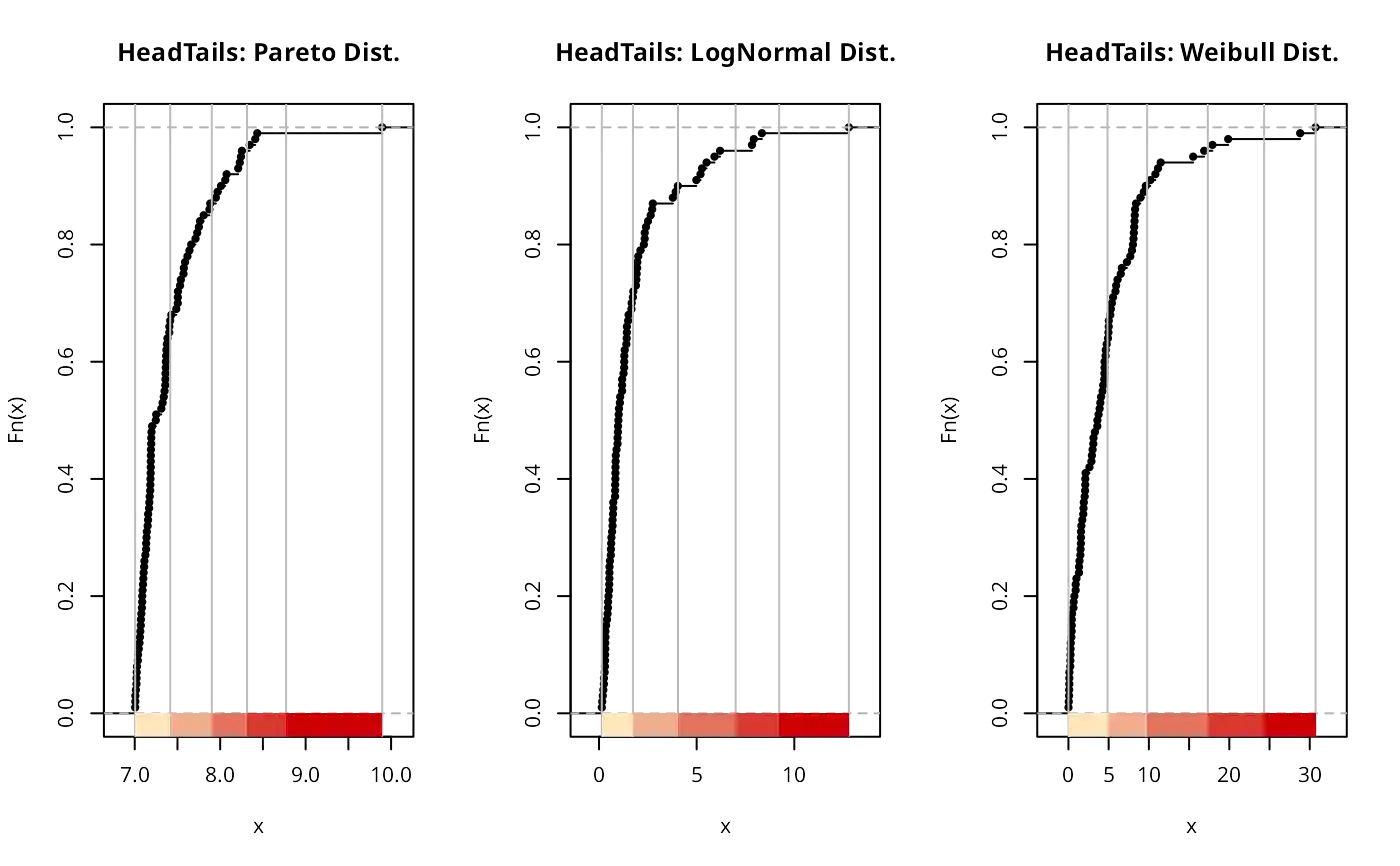
# Head Tails method is suitable for right-sided heavy-tailed distributions
set.seed(1234)
# Heavy tails-----
# Pareto distributions a=7 b=14
paretodist <- 7 / (1 - runif(100)) ^ (1 / 14)
# Lognorm
lognormdist <- rlnorm(100)
# Weibull
weibulldist <- rweibull(100, 1, scale = 5)
pal1 <- c("wheat1", "red3")
opar <- par(mfrow = c(1, 3))
plot(classIntervals(paretodist, style = "headtails"),
pal = pal1,
main = "HeadTails: Pareto Dist.")
plot(classIntervals(lognormdist, style = "headtails"),
pal = pal1,
main = "HeadTails: LogNormal Dist.")
plot(classIntervals(weibulldist, style = "headtails"),
pal = pal1,
main = "HeadTails: Weibull Dist.")
cl2 <- classIntervals(data_censored, n=5, style="jenks", dataPrecision=2)
print(cl2, unique=FALSE)
#> style: jenks
#> one of 4,082,925 possible partitions of this variable into 5 classes
#> [0,0] (0,19.5] (19.5,20.63] (20.63,22.6] (22.6,26]
#> 10 33 39 28 10
print(cl2, unique=TRUE)
#> style: jenks
#> one of 4,082,925 possible partitions of this variable into 5 classes
#> Class found with one single (possibly repeated) value: changed label
#> 0 (0,19.5] (19.5,20.63] (20.63,22.6] 26
#> 10 33 39 28 10
# \dontrun{
set.seed(1)
n <- 1e+05
x <- runif(n)
classIntervals(x, n=5, style="sd")
#> style: sd
#> [-0.07925682,0.06546355) [0.06546355,0.2101839) [0.2101839,0.3549043)
#> 6597 14579 14403
#> [0.3549043,0.4996247) [0.4996247,0.644345) [0.644345,0.7890654)
#> 14395 14446 14439
#> [0.7890654,0.9337858) [0.9337858,1.078506]
#> 14463 6678
classIntervals(x, n=5, style="pretty")
#> style: pretty
#> [0,0.2) [0.2,0.4) [0.4,0.6) [0.6,0.8) [0.8,1]
#> 20142 19936 19888 19993 20041
classIntervals(x, n=5, style="equal")
#> style: equal
#> [3.895489e-06,0.1999925) [0.1999925,0.3999812) [0.3999812,0.5999698)
#> 20141 19935 19888
#> [0.5999698,0.7999584) [0.7999584,0.9999471]
#> 19991 20045
classIntervals(x, n=5, style="quantile")
#> style: quantile
#> [3.895489e-06,0.1984408) [0.1984408,0.3993007) [0.3993007,0.6003913)
#> 20000 20000 20000
#> [0.6003913,0.8003984) [0.8003984,0.9999471]
#> 20000 20000
# the class intervals found vary a little because of sampling
classIntervals(x, n=5, style="kmeans")
#> style: kmeans
#> [3.895489e-06,0.1992885) [0.1992885,0.4002208) [0.4002208,0.600954)
#> 20075 20034 19946
#> [0.600954,0.800892) [0.800892,0.9999471]
#> 20007 19938
classIntervals(x, n=5, style="fisher")
#> Warning: N is large, and some styles will run very slowly; sampling imposed
#> style: fisher
#> [3.895489e-06,0.2084817) [0.2084817,0.4107739) [0.4107739,0.6097159)
#> 21009 20108 19764
#> [0.6097159,0.8037792) [0.8037792,0.9999471]
#> 19470 19649
classIntervals(x, n=5, style="fisher")
#> Warning: N is large, and some styles will run very slowly; sampling imposed
#> style: fisher
#> [3.895489e-06,0.201632) [0.201632,0.4031747) [0.4031747,0.6060818)
#> 20327 20045 20172
#> [0.6060818,0.8071612) [0.8071612,0.9999471]
#> 20159 19297
classIntervals(x, n=5, style="fisher")
#> Warning: N is large, and some styles will run very slowly; sampling imposed
#> style: fisher
#> [3.895489e-06,0.1927805) [0.1927805,0.3880168) [0.3880168,0.5904186)
#> 19443 19489 20059
#> [0.5904186,0.7963362) [0.7963362,0.9999471]
#> 20617 20392
# }
have_units <- FALSE
if (require(units, quietly=TRUE)) have_units <- TRUE
#> udunits database from /usr/share/udunits/udunits2.xml
if (have_units) {
set.seed(1)
x_units <- set_units(sample(seq(1, 100, 0.25), 100), km/h)
# \dontrun{
classIntervals(x_units, n=5, style="sd")
# }
}
#> style: sd
#> one of 14,887,031,544 possible partitions of this [km/h] variable into 8 classes
#> [-6.990949,7.637413) [7.637413,22.26578) [22.26578,36.89414)
#> 6 15 16
#> [36.89414,51.5225) [51.5225,66.15086) [66.15086,80.77922)
#> 12 12 16
#> [80.77922,95.40759) [95.40759,110.0359]
#> 18 5
if (have_units) {
classIntervals(x_units, n=5, style="pretty")
}
#> style: pretty
#> one of 3,764,376 possible partitions of this [km/h] variable into 5 classes
#> [0,20) [20,40) [40,60) [60,80) [80,100]
#> 18 21 19 19 23
if (have_units) {
# \dontrun{
classIntervals(x_units, n=5, style="equal")
# }
}
#> style: equal
#> one of 3,764,376 possible partitions of this [km/h] variable into 5 classes
#> [4,23.1) [23.1,42.2) [42.2,61.3) [61.3,80.4) [80.4,99.5]
#> 22 19 17 19 23
if (have_units) {
classIntervals(x_units, n=5, style="quantile")
}
#> style: quantile
#> one of 3,764,376 possible partitions of this [km/h] variable into 5 classes
#> [4,21.95) [21.95,41.5) [41.5,64.05) [64.05,82.8) [82.8,99.5]
#> 20 20 20 20 20
if (have_units) {
# \dontrun{
classIntervals(x_units, n=5, style="kmeans")
# }
}
#> style: kmeans
#> one of 3,764,376 possible partitions of this [km/h] variable into 5 classes
#> [4,19.375) [19.375,39.375) [39.375,60.5) [60.5,79.625) [79.625,99.5]
#> 18 21 19 19 23
if (have_units) {
classIntervals(x_units, n=5, style="fisher")
}
#> style: fisher
#> one of 3,764,376 possible partitions of this [km/h] variable into 5 classes
#> [4,19.375) [19.375,39.375) [39.375,60.5) [60.5,79.625) [79.625,99.5]
#> 18 21 19 19 23
if (have_units) {
classIntervals(x_units, style="headtails")
}
#> style: headtails
#> one of 99 possible partitions of this [km/h] variable into 2 classes
#> [4,51.5225) [51.5225,99.5]
#> 49 51
if (have_units) {
classIntervals(x_units, style="box")
}
#> style: box
#> one of 71,523,144 possible partitions of this [km/h] variable into 6 classes
#> [-Inf,-46.375) [-46.375,26.9375) [26.9375,52) [52,75.8125)
#> 0 25 25 25
#> [75.8125,149.125) [149.125,Inf]
#> 25 0
# \dontrun{
st <- Sys.time()
x_POSIXt <- sample(st+((0:500)*3600), 100)
fx <- st+((0:5)*3600)*100
classIntervals(x_POSIXt, style="fixed", fixedBreaks=fx)
#> style: fixed
#> one of 3,764,376 possible partitions of this variable into 5 classes
#> [2024-12-27 10:41:00.252928,2024-12-31 14:41:00.252928)
#> 21
#> [2024-12-31 14:41:00.252928,2025-01-04 18:41:00.252928)
#> 18
#> [2025-01-04 18:41:00.252928,2025-01-08 22:41:00.252928)
#> 19
#> [2025-01-08 22:41:00.252928,2025-01-13 02:41:00.252928)
#> 21
#> [2025-01-13 02:41:00.252928,2025-01-17 06:41:00.252928]
#> 21
classIntervals(x_POSIXt, n=5, style="sd")
#> style: sd
#> one of 14,887,031,544 possible partitions of this variable into 8 classes
#> [2024-12-25 13:40:28.307138,2024-12-28 14:46:36.293586)
#> 5
#> [2024-12-28 14:46:36.293586,2024-12-31 15:52:44.280033)
#> 16
#> [2024-12-31 15:52:44.280033,2025-01-03 16:58:52.266481)
#> 17
#> [2025-01-03 16:58:52.266481,2025-01-06 18:05:00.252928)
#> 12
#> [2025-01-06 18:05:00.252928,2025-01-09 19:11:08.239376)
#> 14
#> [2025-01-09 19:11:08.239376,2025-01-12 20:17:16.225824)
#> 14
#> [2025-01-12 20:17:16.225824,2025-01-15 21:23:24.212271)
#> 16
#> [2025-01-15 21:23:24.212271,2025-01-18 22:29:32.19871]
#> 6
classIntervals(x_POSIXt, n=5, style="pretty")
#> style: pretty
#> one of 3,764,376 possible partitions of this variable into 5 classes
#> [2024-12-24 01:26:40,2024-12-29 20:20:00)
#> 12
#> [2024-12-29 20:20:00,2025-01-04 15:13:20)
#> 27
#> [2025-01-04 15:13:20,2025-01-10 10:06:40)
#> 28
#> [2025-01-10 10:06:40,2025-01-16 05:00:00)
#> 28
#> [2025-01-16 05:00:00,2025-01-21 23:53:20]
#> 5
classIntervals(x_POSIXt, n=5, style="equal")
#> style: equal
#> one of 3,764,376 possible partitions of this variable into 5 classes
#> [2024-12-27 23:41:00.252928,2025-01-01 00:05:00.252928)
#> 23
#> [2025-01-01 00:05:00.252928,2025-01-05 00:29:00.252928)
#> 16
#> [2025-01-05 00:29:00.252928,2025-01-09 00:53:00.252928)
#> 19
#> [2025-01-09 00:53:00.252928,2025-01-13 01:17:00.252928)
#> 20
#> [2025-01-13 01:17:00.252928,2025-01-17 01:41:00.252928]
#> 22
classIntervals(x_POSIXt, n=5, style="quantile")
#> style: quantile
#> one of 3,764,376 possible partitions of this variable into 5 classes
#> [2024-12-27 23:41:00.252928,2024-12-31 10:29:00.252928)
#> 20
#> [2024-12-31 10:29:00.252928,2025-01-05 03:41:00.252928)
#> 20
#> [2025-01-05 03:41:00.252928,2025-01-09 03:05:00.252928)
#> 20
#> [2025-01-09 03:05:00.252928,2025-01-13 05:17:00.252928)
#> 20
#> [2025-01-13 05:17:00.252928,2025-01-17 01:41:00.252928]
#> 20
classIntervals(x_POSIXt, n=5, style="kmeans")
#> style: kmeans
#> one of 3,764,376 possible partitions of this variable into 5 classes
#> [2024-12-27 23:41:00.252928,2024-12-31 02:41:00.252928)
#> 19
#> [2024-12-31 02:41:00.252928,2025-01-04 01:41:00.252928)
#> 19
#> [2025-01-04 01:41:00.252928,2025-01-08 10:11:00.252928)
#> 17
#> [2025-01-08 10:11:00.252928,2025-01-12 14:11:00.252928)
#> 23
#> [2025-01-12 14:11:00.252928,2025-01-17 01:41:00.252928]
#> 22
classIntervals(x_POSIXt, n=5, style="fisher")
#> style: fisher
#> one of 3,764,376 possible partitions of this variable into 5 classes
#> [2024-12-27 23:41:00.252928,2024-12-31 02:41:00.252928)
#> 19
#> [2024-12-31 02:41:00.252928,2025-01-04 01:41:00.252928)
#> 19
#> [2025-01-04 01:41:00.252928,2025-01-08 10:11:00.252928)
#> 17
#> [2025-01-08 10:11:00.252928,2025-01-12 14:11:00.252928)
#> 23
#> [2025-01-12 14:11:00.252928,2025-01-17 01:41:00.252928]
#> 22
classIntervals(x_POSIXt, style="headtails")
#> style: headtails
#> one of 99 possible partitions of this variable into 2 classes
#> [2024-12-27 23:41:00.252928,2025-01-06 18:05:00.252928)
#> 50
#> [2025-01-06 18:05:00.252928,2025-01-17 01:41:00.252928]
#> 50
classIntervals(x_POSIXt, style="maximum")
#> style: maximum
#> one of 14,887,031,544 possible partitions of this variable into 8 classes
#> [2024-12-27 23:41:00.252928,2025-01-03 08:41:00.252928)
#> 37
#> [2025-01-03 08:41:00.252928,2025-01-04 01:41:00.252928)
#> 1
#> [2025-01-04 01:41:00.252928,2025-01-04 18:11:00.252928)
#> 1
#> [2025-01-04 18:11:00.252928,2025-01-07 02:41:00.252928)
#> 12
#> [2025-01-07 02:41:00.252928,2025-01-10 09:41:00.252928)
#> 16
#> [2025-01-10 09:41:00.252928,2025-01-12 14:11:00.252928)
#> 11
#> [2025-01-12 14:11:00.252928,2025-01-15 22:11:00.252928)
#> 16
#> [2025-01-15 22:11:00.252928,2025-01-17 01:41:00.252928]
#> 6
classIntervals(x_POSIXt, style="box")
#> style: box
#> one of 71,523,144 possible partitions of this variable into 6 classes
#> [-Inf,2024-12-17 03:03:30.252928)
#> 0
#> [2024-12-17 03:03:30.252928,2025-01-01 10:11:00.252928)
#> 25
#> [2025-01-01 10:11:00.252928,2025-01-06 17:41:00.252928)
#> 25
#> [2025-01-06 17:41:00.252928,2025-01-11 14:56:00.252928)
#> 25
#> [2025-01-11 14:56:00.252928,2025-01-26 22:03:30.252928)
#> 25
#> [2025-01-26 22:03:30.252928,Inf]
#> 0
# }
# see vignette for further details
# \dontrun{
# Head Tails method is suitable for right-sided heavy-tailed distributions
set.seed(1234)
# Heavy tails-----
# Pareto distributions a=7 b=14
paretodist <- 7 / (1 - runif(100)) ^ (1 / 14)
# Lognorm
lognormdist <- rlnorm(100)
# Weibull
weibulldist <- rweibull(100, 1, scale = 5)
pal1 <- c("wheat1", "red3")
opar <- par(mfrow = c(1, 3))
plot(classIntervals(paretodist, style = "headtails"),
pal = pal1,
main = "HeadTails: Pareto Dist.")
plot(classIntervals(lognormdist, style = "headtails"),
pal = pal1,
main = "HeadTails: LogNormal Dist.")
plot(classIntervals(weibulldist, style = "headtails"),
pal = pal1,
main = "HeadTails: Weibull Dist.")
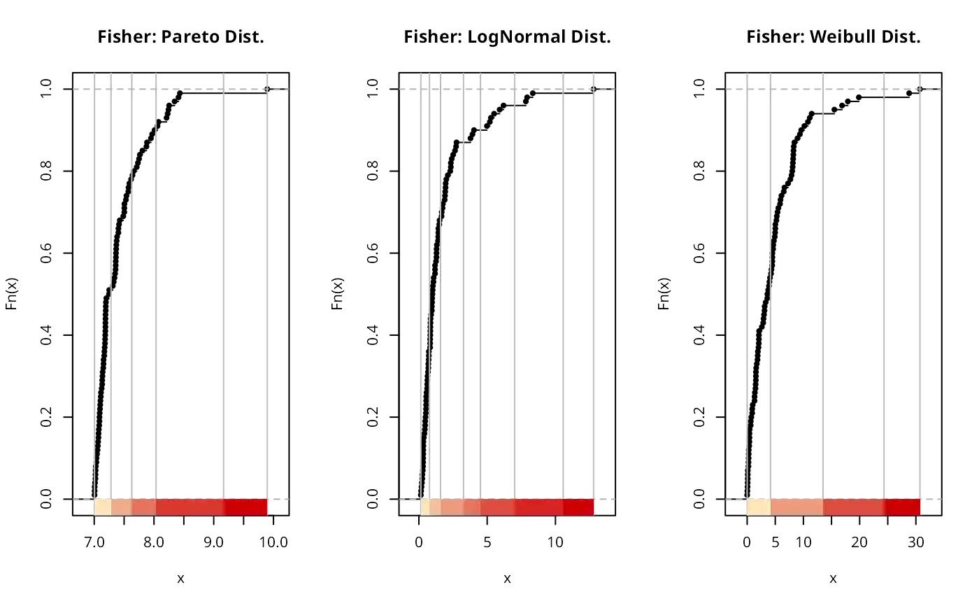
 plot(classIntervals(paretodist, n = 5, style = "fisher"),
pal = pal1,
main = "Fisher: Pareto Dist.")
plot(classIntervals(lognormdist, n = 7, style = "fisher"),
pal = pal1,
main = "Fisher: LogNormal Dist.")
plot(classIntervals(weibulldist, n= 4, style = "fisher"),
pal = pal1,
main = "Fisher: Weibull Dist.")
plot(classIntervals(paretodist, n = 5, style = "fisher"),
pal = pal1,
main = "Fisher: Pareto Dist.")
plot(classIntervals(lognormdist, n = 7, style = "fisher"),
pal = pal1,
main = "Fisher: LogNormal Dist.")
plot(classIntervals(weibulldist, n= 4, style = "fisher"),
pal = pal1,
main = "Fisher: Weibull Dist.")
 par(opar)
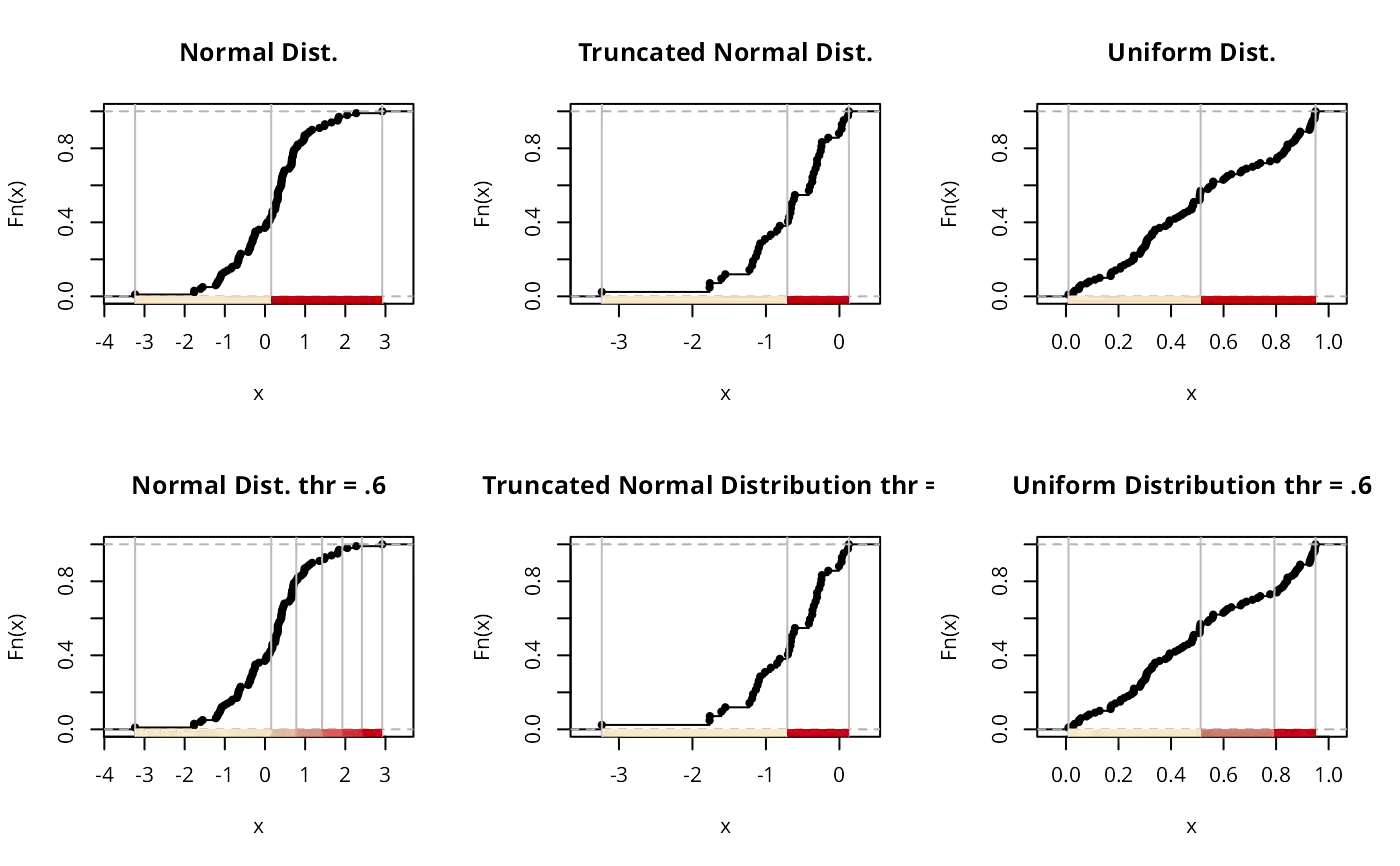
#Non heavy tails, thr should be increased-----
#Normal dist
normdist <- rnorm(100)
#Left-tailed truncated Normal distr
leftnorm <- rep(normdist[normdist < mean(normdist)], 2)
# Uniform distribution
unifdist <- runif(100)
opar <- par(mfrow = c(2, 3))
plot(classIntervals(normdist, style = "headtails"),
pal = pal1,
main = "Normal Dist.")
plot(classIntervals(leftnorm, style = "headtails"),
pal = pal1,
main = "Truncated Normal Dist.")
plot(classIntervals(unifdist, style = "headtails"),
pal = pal1,
main = "Uniform Dist.")
# thr should be increased for non heavy-tailed distributions
plot(
classIntervals(normdist, style = "headtails", thr = .6),
pal = pal1,
main = "Normal Dist. thr = .6"
)
plot(
classIntervals(leftnorm, style = "headtails", thr = .6),
pal = pal1,
main = "Truncated Normal Distribution thr = .6"
)
plot(
classIntervals(unifdist, style = "headtails", thr = .6),
pal = pal1,
main = "Uniform Distribution thr = .6"
)
par(opar)
#Non heavy tails, thr should be increased-----
#Normal dist
normdist <- rnorm(100)
#Left-tailed truncated Normal distr
leftnorm <- rep(normdist[normdist < mean(normdist)], 2)
# Uniform distribution
unifdist <- runif(100)
opar <- par(mfrow = c(2, 3))
plot(classIntervals(normdist, style = "headtails"),
pal = pal1,
main = "Normal Dist.")
plot(classIntervals(leftnorm, style = "headtails"),
pal = pal1,
main = "Truncated Normal Dist.")
plot(classIntervals(unifdist, style = "headtails"),
pal = pal1,
main = "Uniform Dist.")
# thr should be increased for non heavy-tailed distributions
plot(
classIntervals(normdist, style = "headtails", thr = .6),
pal = pal1,
main = "Normal Dist. thr = .6"
)
plot(
classIntervals(leftnorm, style = "headtails", thr = .6),
pal = pal1,
main = "Truncated Normal Distribution thr = .6"
)
plot(
classIntervals(unifdist, style = "headtails", thr = .6),
pal = pal1,
main = "Uniform Distribution thr = .6"
)
 par(opar)
# }
par(opar)
# }