4.3. Style Advanced — Python
4.3.1. Label rotation
Code 4.7. Label rotation
import matplotlib.pyplot as plt

x = [1, 2, 3, 4]
y = [1, 4, 9, 6]
labels = ['Frogs', 'Hogs', 'Bogs', 'Slogs']

plt.plot(x, y, 'ro')

# You can specify a rotation for the tick labels in degrees or with keywords.
plt.xticks(rotation=45)

# Pad margins so that markers don't get clipped by the axes
plt.margins(0.2)

# Tweak spacing to prevent clipping of tick-labels
plt.subplots_adjust(bottom=0.15)
plt.show()
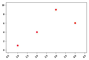
Figure 4.22. Label rotation
4.3.2. Grid
Code 4.8. Grid Simple
import matplotlib.pyplot as plt

x = [1, 2, 3, 4, 5]
y = [1, 2, 3, 4, 5]
plt.plot(x, y)


plt.grid(True)
plt.show()
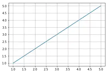
Figure 4.23. Grid Simple
Code 4.9. Grid Extra
import numpy as np
import matplotlib.pyplot as plt

fig = plt.figure()
ax = fig.add_subplot(1, 1, 1)

# Major ticks every 20, minor ticks every 5
major_ticks = np.arange(0, 101, 20)
minor_ticks = np.arange(0, 101, 5)

ax.set_xticks(major_ticks)
ax.set_xticks(minor_ticks, minor=True)
ax.set_yticks(major_ticks)
ax.set_yticks(minor_ticks, minor=True)

# And a corresponding grid
ax.grid(which='both')

# Or if you want different settings for the grids:
ax.grid(which='minor', alpha=0.2)
ax.grid(which='major', alpha=0.5)

plt.show()
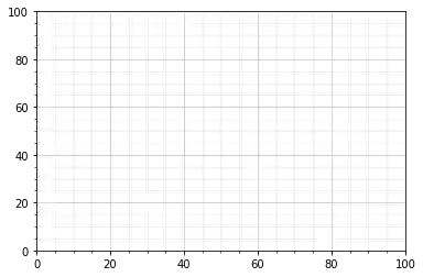
Figure 4.24. Grid Extra
4.3.3. Trend line
Code 4.10. Trend line
import matplotlib.pylab as pylab
import numpy as np

x = [1, 3, 5, 7, 9]
y = [2, 3, 4, 3, 4]

# plot the data itself
pylab.plot(x, y, label="data")

# calc the trendline (it is simply a linear fitting)
z = np.polyfit(x, y, 1)
p = np.poly1d(z)

pylab.plot(x, p(x), color="red", linestyle='--')

# the line equation:
a = z[0]
b = z[1]
print(f"y = {a:.6}x + ({b:.6})")

# parabolic fit will be:
# z = numpy.polyfit(x, y, 2)
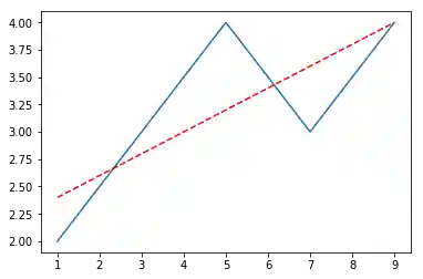
Figure 4.25. Trend line
4.3.4. Error bars
Code 4.11. Error bars
import matplotlib.pyplot as plt

x = [1, 2, 3, 4]
y = [1, 4, 9, 16]
e = [0.5, 1., 1.5, 2.]

plt.errorbar(x, y, yerr=e, fmt='o')
plt.show()
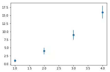
Figure 4.26. Error bars
4.3.5. Colorbar
Code 4.12. Colorbar
from matplotlib import pyplot as plt
from sklearn.datasets import load_iris


iris = load_iris()

# The indices of the features that we are plotting
x_index = 0
y_index = 1

# this formatter will label the `colorbar` with the correct target names
formatter = plt.FuncFormatter(lambda i, *args: iris.target_names[int(i)])

plt.figure(figsize=(5, 4))
plt.scatter(iris.data[:, x_index], iris.data[:, y_index], c=iris.target)
plt.colorbar(ticks=[0, 1, 2], format=formatter)

plt.xlabel(iris.feature_names[x_index])
plt.ylabel(iris.feature_names[y_index])

plt.tight_layout()
plt.show()
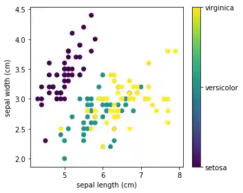
Figure 4.27. Colorbar
4.3.6. Changing colors
ax.spines['bottom'].set_color('#dddddd')
ax.spines['top'].set_color('#dddddd')
ax.spines['right'].set_color('red')
ax.spines['left'].set_color('red')
ax.tick_params(axis='x', colors='red')
ax.tick_params(axis='y', colors='red')
ax.yaxis.label.set_color('red')
ax.xaxis.label.set_color('red')
ax.title.set_color('red')
4.3.7. Using mathematical expressions in text
plt.title(r'$\sigma_i=15$')
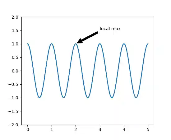
4.3.8. Annotations
4.3.9. Single Annotation
import matplotlib.pyplot as plt
import numpy as np

ax = plt.subplot(111)

t = np.arange(0.0, 5.0, 0.01)
s = np.cos(2*np.pi*t)
line, = plt.plot(t, s, lw=2)

plt.annotate('local max',
    xy=(2, 1),
    xytext=(3, 1.5),
    arrowprops={'facecolor': 'black', 'shrink': 0.05},
)

plt.ylim(-2,2)
plt.show()  # doctest: +SKIP
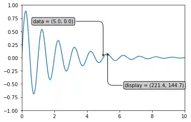
4.3.10. Multiple Annotations
Code 4.13. Multiple Annotations
import numpy as np
import matplotlib.pyplot as plt

x = np.arange(0, 10, 0.005)
y = np.exp(-x / 2.) * np.sin(2 * np.pi * x)

fig = plt.figure()
ax = fig.add_subplot(111)
ax.plot(x, y)
ax.set_xlim(0, 10)
ax.set_ylim(-1, 1)


data_x = 5
data_y = 0
display_x, display_y = ax.transData.transform_point((data_x, data_y))

bbox = dict(boxstyle="round", fc="0.8")
arrowprops = dict(
    arrowstyle="->",
    connectionstyle="angle,angleA=0,angleB=90,rad=10")

offset = 72
ax.annotate('data = (%.1f, %.1f)' % (data_x, data_y),
            (data_x, data_y), xytext=(-2 * offset, offset), textcoords='offset points',
            bbox=bbox, arrowprops=arrowprops)

display = ax.annotate('display = (%.1f, %.1f)' % (display_x, display_y),
                      (display_x, display_y), xytext=(0.5 * offset, -offset),
                      xycoords='figure pixels',
                      textcoords='offset points',
                      bbox=bbox, arrowprops=arrowprops)

plt.show()