Different gradient computations for regularized optimal transport — POT Python Optimal Transport 0.9.6 documentation
Note
Go to the end to download the full example code.
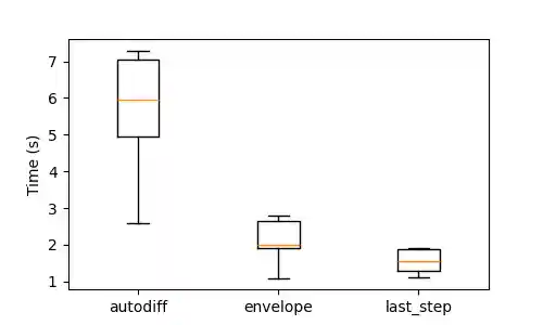
This example illustrates the differences in terms of computation time between the gradient options for the Sinkhorn solver.
Note
Example added in release: 0.9.6
# Author: Sonia Mazelet <sonia.mazelet@polytechnique.edu>
#
# License: MIT License

# sphinx_gallery_thumbnail_number = 1

import matplotlib.pylab as pl
import ot
from ot.backend import torch
Time comparison of the Sinkhorn solver for different gradient options
n_trials = 10
times_autodiff = torch.zeros(n_trials)
times_envelope = torch.zeros(n_trials)
times_last_step = torch.zeros(n_trials)

n_samples_s = 300
n_samples_t = 300
n_features = 5
reg = 0.03

# Time required for the Sinkhorn solver and gradient computations, for different gradient options over multiple Gaussian distributions
for i in range(n_trials):
    x = torch.rand((n_samples_s, n_features))
    y = torch.rand((n_samples_t, n_features))
    a = ot.utils.unif(n_samples_s)
    b = ot.utils.unif(n_samples_t)
    M = ot.dist(x, y)

    a = torch.tensor(a, requires_grad=True)
    b = torch.tensor(b, requires_grad=True)
    M = M.clone().detach().requires_grad_(True)

    # autodiff provides the gradient for all the outputs (plan, value, value_linear)
    ot.tic()
    res_autodiff = ot.solve(M, a, b, reg=reg, grad="autodiff")
    res_autodiff.value.backward()
    times_autodiff[i] = ot.toq()

    a = a.clone().detach().requires_grad_(True)
    b = b.clone().detach().requires_grad_(True)
    M = M.clone().detach().requires_grad_(True)

    # envelope provides the gradient for value
    ot.tic()
    res_envelope = ot.solve(M, a, b, reg=reg, grad="envelope")
    res_envelope.value.backward()
    times_envelope[i] = ot.toq()

    a = a.clone().detach().requires_grad_(True)
    b = b.clone().detach().requires_grad_(True)
    M = M.clone().detach().requires_grad_(True)

    # last_step provides the gradient for all the outputs, but only for the last iteration of the Sinkhorn algorithm
    ot.tic()
    res_last_step = ot.solve(M, a, b, reg=reg, grad="last_step")
    res_last_step.value.backward()
    times_last_step[i] = ot.toq()

pl.figure(1, figsize=(5, 3))
pl.ticklabel_format(axis="y", style="sci", scilimits=(0, 0))
pl.boxplot(
    ([times_autodiff, times_envelope, times_last_step]),
    tick_labels=["autodiff", "envelope", "last_step"],
    showfliers=False,
)
pl.ylabel("Time (s)")
pl.show()
Total running time of the script: (1 minutes 43.524 seconds)