Linear OT mapping estimation — POT Python Optimal Transport 0.9.6 documentation
Note
Go to the end to download the full example code.
Note
Example updated in release: 0.9.1.
# Author: Remi Flamary <remi.flamary@unice.fr>
#
# License: MIT License

# sphinx_gallery_thumbnail_number = 2
import os
from pathlib import Path

import numpy as np
from matplotlib import pyplot as plt
import ot
Generate data
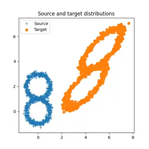
n = 1000
d = 2
sigma = 0.1

rng = np.random.RandomState(42)

# source samples
angles = rng.rand(n, 1) * 2 * np.pi
xs = np.concatenate((np.sin(angles), np.cos(angles)), axis=1) + sigma * rng.randn(n, 2)
xs[: n // 2, 1] += 2


# target samples
anglet = rng.rand(n, 1) * 2 * np.pi
xt = np.concatenate((np.sin(anglet), np.cos(anglet)), axis=1) + sigma * rng.randn(n, 2)
xt[: n // 2, 1] += 2


A = np.array([[1.5, 0.7], [0.7, 1.5]])
b = np.array([[4, 2]])
xt = xt.dot(A) + b
Plot data
plt.figure(1, (5, 5))
plt.plot(xs[:, 0], xs[:, 1], "+")
plt.plot(xt[:, 0], xt[:, 1], "o")
plt.legend(("Source", "Target"))
plt.title("Source and target distributions")
plt.show()
Estimate linear mapping and transport
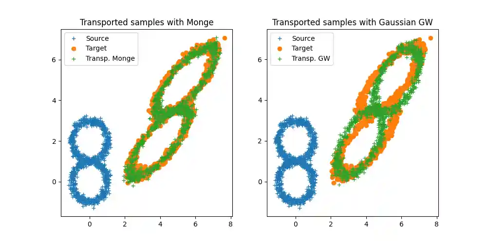
Plot transported samples
plt.figure(2, (10, 5))
plt.clf()
plt.subplot(1, 2, 1)
plt.plot(xs[:, 0], xs[:, 1], "+")
plt.plot(xt[:, 0], xt[:, 1], "o")
plt.plot(xst[:, 0], xst[:, 1], "+")
plt.legend(("Source", "Target", "Transp. Monge"), loc=0)
plt.title("Transported samples with Monge")
plt.subplot(1, 2, 2)
plt.plot(xs[:, 0], xs[:, 1], "+")
plt.plot(xt[:, 0], xt[:, 1], "o")
plt.plot(xstgw[:, 0], xstgw[:, 1], "+")
plt.legend(("Source", "Target", "Transp. GW"), loc=0)
plt.title("Transported samples with Gaussian GW")
plt.show()
Load image data
Estimate mapping and adapt
Plot transformed images
plt.figure(3, figsize=(14, 7))

plt.subplot(2, 3, 1)
plt.imshow(I1)
plt.axis("off")
plt.title("Im. 1")

plt.subplot(2, 3, 4)
plt.imshow(I2)
plt.axis("off")
plt.title("Im. 2")

plt.subplot(2, 3, 2)
plt.imshow(I1t)
plt.axis("off")
plt.title("Monge mapping Im. 1")

plt.subplot(2, 3, 5)
plt.imshow(I2t)
plt.axis("off")
plt.title("Inverse Monge mapping Im. 2")

plt.subplot(2, 3, 3)
plt.imshow(I1tgw)
plt.axis("off")
plt.title("Gaussian GW mapping Im. 1")

plt.subplot(2, 3, 6)
plt.imshow(I2tgw)
plt.axis("off")
plt.title("Inverse Gaussian GW mapping Im. 2")

Text(0.5, 1.0, 'Inverse Gaussian GW mapping Im. 2')
Total running time of the script: (0 minutes 2.175 seconds)