OTDA unsupervised vs semi-supervised setting — POT Python Optimal Transport 0.9.6 documentation
Note
Go to the end to download the full example code.
Note
Example added in release: 0.1.9.
This example introduces a semi supervised domain adaptation in a 2D setting. It explicit the problem of semi supervised domain adaptation and introduces some optimal transport approaches to solve it.
Quantities such as optimal couplings, greater coupling coefficients and transported samples are represented in order to give a visual understanding of what the transport methods are doing.
# Authors: Remi Flamary <remi.flamary@unice.fr>
#          Stanislas Chambon <stan.chambon@gmail.com>
#
# License: MIT License

# sphinx_gallery_thumbnail_number = 3

import matplotlib.pylab as pl
import ot
Generate data
Transport source samples onto target samples
Fig 1 : plots source and target samples + matrix of pairwise distance
pl.figure(1, figsize=(10, 10))
pl.subplot(2, 2, 1)
pl.scatter(Xs[:, 0], Xs[:, 1], c=ys, marker="+", label="Source samples")
pl.xticks([])
pl.yticks([])
pl.legend(loc=0)
pl.title("Source  samples")

pl.subplot(2, 2, 2)
pl.scatter(Xt[:, 0], Xt[:, 1], c=yt, marker="o", label="Target samples")
pl.xticks([])
pl.yticks([])
pl.legend(loc=0)
pl.title("Target samples")

pl.subplot(2, 2, 3)
pl.imshow(ot_sinkhorn_un.cost_, interpolation="nearest")
pl.xticks([])
pl.yticks([])
pl.title("Cost matrix - unsupervised DA")

pl.subplot(2, 2, 4)
pl.imshow(ot_sinkhorn_semi.cost_, interpolation="nearest")
pl.xticks([])
pl.yticks([])
pl.title("Cost matrix - semi-supervised DA")

pl.tight_layout()

# the optimal coupling in the semi-supervised DA case will exhibit " shape
# similar" to the cost matrix, (block diagonal matrix)
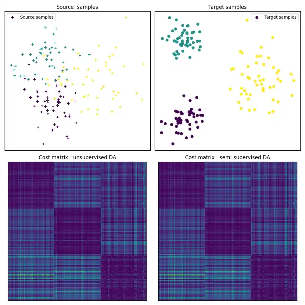
Fig 2 : plots optimal couplings for the different methods
pl.figure(2, figsize=(8, 4))

pl.subplot(1, 2, 1)
pl.imshow(ot_sinkhorn_un.coupling_, interpolation="nearest", cmap="gray_r")
pl.xticks([])
pl.yticks([])
pl.title("Optimal coupling\nUnsupervised DA")

pl.subplot(1, 2, 2)
pl.imshow(ot_sinkhorn_semi.coupling_, interpolation="nearest", cmap="gray_r")
pl.xticks([])
pl.yticks([])
pl.title("Optimal coupling\nSemi-supervised DA")

pl.tight_layout()
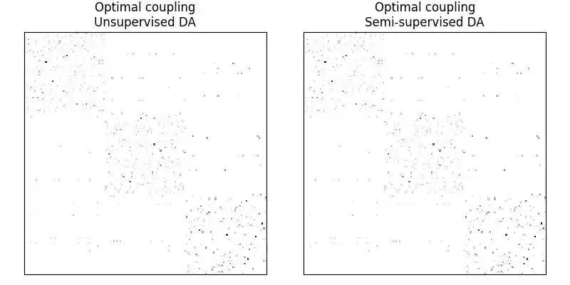
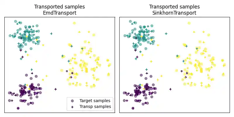
Fig 3 : plot transported samples
# display transported samples
pl.figure(4, figsize=(8, 4))
pl.subplot(1, 2, 1)
pl.scatter(Xt[:, 0], Xt[:, 1], c=yt, marker="o", label="Target samples", alpha=0.5)
pl.scatter(
    transp_Xs_sinkhorn_un[:, 0],
    transp_Xs_sinkhorn_un[:, 1],
    c=ys,
    marker="+",
    label="Transp samples",
    s=30,
)
pl.title("Transported samples\nEmdTransport")
pl.legend(loc=0)
pl.xticks([])
pl.yticks([])

pl.subplot(1, 2, 2)
pl.scatter(Xt[:, 0], Xt[:, 1], c=yt, marker="o", label="Target samples", alpha=0.5)
pl.scatter(
    transp_Xs_sinkhorn_semi[:, 0],
    transp_Xs_sinkhorn_semi[:, 1],
    c=ys,
    marker="+",
    label="Transp samples",
    s=30,
)
pl.title("Transported samples\nSinkhornTransport")
pl.xticks([])
pl.yticks([])

pl.tight_layout()
pl.show()
Total running time of the script: (0 minutes 1.510 seconds)