This example is designed to show how to use SSNB [58] in POT. SSNB computes an l-strongly convex potential \(\varphi\) with an L-Lipschitz gradient such that \(\nabla \varphi \# \mu \approx \nu\). This regularity can be enforced only on the components of a partition of the ambient space, which is a relaxation compared to imposing global regularity.

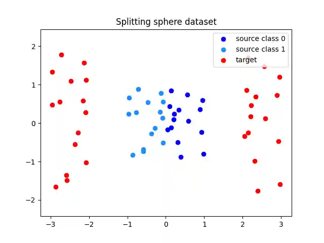
In this example, we consider a source measure \(\mu_s\) which is the uniform measure on the unit square in \(\mathbb{R}^2\), and the target measure \(\mu_t\) which is the image of \(\mu_x\) by \(T(x_1, x_2) = (x_1 + 2\mathrm{sign}(x_2), 2 * x_2)\). The map \(T\) is non-smooth, and we wish to approximate it using a “Brenier-style” map \(\nabla \varphi\) which is regular on the partition \(\lbrace x_1 <=0, x_1>0\rbrace\), which is well adapted to this particular dataset.

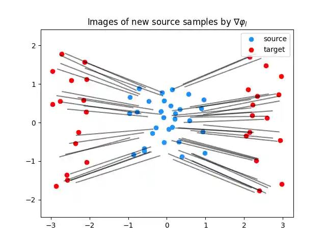
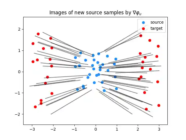
We represent the gradients of the “bounding potentials” \(\varphi_l, \varphi_u\) (from [59], Theorem 3.14), which bound any SSNB potential which is optimal in the sense of [58], Definition 1:

\[\varphi \in \mathrm{argmin}_{\varphi \in \mathcal{F}}\ \mathrm{W}_2(\nabla \varphi \#\mu_s, \mu_t),\]

where \(\mathcal{F}\) is the space functions that are on every set \(E_k\) l-strongly convex with an L-Lipschitz gradient, given \((E_k)_{k \in [K]}\) a partition of the ambient source space.

We perform the optimisation on a low amount of fitting samples and with few iterations, since solving the SSNB problem is quite computationally expensive.

THIS EXAMPLE REQUIRES CVXPY

# Author: Eloi Tanguy <eloi.tanguy@math.cnrs.fr>
# License: MIT License

# sphinx_gallery_thumbnail_number = 3

import matplotlib.pyplot as plt
import numpy as np
import ot

Generating the fitting data

n_fitting_samples = 30
rng = np.random.RandomState(seed=0)
Xs = rng.uniform(-1, 1, size=(n_fitting_samples, 2))
Xs_classes = (Xs[:, 0] < 0).astype(int)
Xt = np.stack([Xs[:, 0] + 2 * np.sign(Xs[:, 0]), 2 * Xs[:, 1]], axis=-1)

plt.scatter(
    Xs[Xs_classes == 0, 0], Xs[Xs_classes == 0, 1], c="blue", label="source class 0"
)
plt.scatter(
    Xs[Xs_classes == 1, 0],
    Xs[Xs_classes == 1, 1],
    c="dodgerblue",
    label="source class 1",
)
plt.scatter(Xt[:, 0], Xt[:, 1], c="red", label="target")
plt.axis("equal")
plt.title("Splitting sphere dataset")
plt.legend(loc="upper right")
plt.show()

Fitting the Nearest Brenier Potential

Plotting the images of the source data

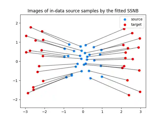
plt.clf()
plt.scatter(Xs[:, 0], Xs[:, 1], c="dodgerblue", label="source")
plt.scatter(Xt[:, 0], Xt[:, 1], c="red", label="target")
for i in range(n_fitting_samples):
    plt.plot([Xs[i, 0], G[i, 0]], [Xs[i, 1], G[i, 1]], color="black", alpha=0.5)
plt.title("Images of in-data source samples by the fitted SSNB")
plt.legend(loc="upper right")
plt.axis("equal")
plt.show()

Computing the predictions (images by nabla phi) for random samples of the source distribution

n_predict_samples = 50
Ys = rng.uniform(-1, 1, size=(n_predict_samples, 2))
Ys_classes = (Ys[:, 0] < 0).astype(int)
phi_lu, G_lu = ot.mapping.nearest_brenier_potential_predict_bounds(
    Xs, phi, G, Ys, Xs_classes, Ys_classes, gradient_lipschitz_constant=L
)

Plot predictions for the gradient of the lower-bounding potential

plt.clf()
plt.scatter(Xs[:, 0], Xs[:, 1], c="dodgerblue", label="source")
plt.scatter(Xt[:, 0], Xt[:, 1], c="red", label="target")
for i in range(n_predict_samples):
    plt.plot(
        [Ys[i, 0], G_lu[0, i, 0]], [Ys[i, 1], G_lu[0, i, 1]], color="black", alpha=0.5
    )
plt.title("Images of new source samples by $\\nabla \\varphi_l$")
plt.legend(loc="upper right")
plt.axis("equal")
plt.show()

Plot predictions for the gradient of the upper-bounding potential

plt.clf()
plt.scatter(Xs[:, 0], Xs[:, 1], c="dodgerblue", label="source")
plt.scatter(Xt[:, 0], Xt[:, 1], c="red", label="target")
for i in range(n_predict_samples):
    plt.plot(
        [Ys[i, 0], G_lu[1, i, 0]], [Ys[i, 1], G_lu[1, i, 1]], color="black", alpha=0.5
    )
plt.title("Images of new source samples by $\\nabla \\varphi_u$")
plt.legend(loc="upper right")
plt.axis("equal")
plt.show()

Total running time of the script: (0 minutes 57.478 seconds)

Gallery generated by Sphinx-Gallery