Learning sample marginal distribution with CO-Optimal Transport — POT Python Optimal Transport 0.9.4 documentation
Note
Go to the end to download the full example code.
In this example, we illustrate how to estimate the sample marginal distribution which minimizes the CO-Optimal Transport distance [47]_ between two matrices. More precisely, given a source data \((X, \mu_x^{(s)}, \mu_x^{(f)})\) and a target matrix \(Y\) associated with a fixed histogram on features \(\mu_y^{(f)}\), we want to solve the following problem
\[\min_{\mu_y^{(s)} \in \Delta} \text{COOT}\left( (X, \mu_x^{(s)}, \mu_x^{(f)}), (Y, \mu_y^{(s)}, \mu_y^{(f)}) \right)\]
where \(\Delta\) is the probability simplex. This minimization is done with a
simple projected gradient descent in PyTorch. We use the automatic backend of POT that
allows us to compute the CO-Optimal Transport distance with ot.coot.co_optimal_transport2()
with differentiable losses.
# Author: Remi Flamary <remi.flamary@unice.fr>
#         Quang Huy Tran <quang-huy.tran@univ-ubs.fr>
# License: MIT License

from matplotlib.patches import ConnectionPatch
import torch
import numpy as np

import matplotlib.pyplot as pl
import ot

from ot.coot import co_optimal_transport as coot
from ot.coot import co_optimal_transport2 as coot2
Generate data
The source and clean target matrices are generated by \(X_{i,j} = \cos(\frac{i}{n_1} \pi) + \cos(\frac{j}{d_1} \pi)\) and \(Y_{i,j} = \cos(\frac{i}{n_2} \pi) + \cos(\frac{j}{d_2} \pi)\). The target matrix is then contaminated by adding 5 row outliers. Intuitively, we expect that the estimated sample distribution should ignore these outliers, i.e. their weights should be zero.
np.random.seed(182)

n1, d1 = 20, 16
n2, d2 = 10, 8
n = 15

X = (
    torch.cos(torch.arange(n1) * torch.pi / n1)[:, None] +
    torch.cos(torch.arange(d1) * torch.pi / d1)[None, :]
)

# Generate clean target data mixed with outliers
Y_noisy = torch.randn((n, d2)) * 10.0
Y_noisy[:n2, :] = (
    torch.cos(torch.arange(n2) * torch.pi / n2)[:, None] +
    torch.cos(torch.arange(d2) * torch.pi / d2)[None, :]
)
Y = Y_noisy[:n2, :]

X, Y_noisy, Y = X.double(), Y_noisy.double(), Y.double()

fig, axes = pl.subplots(nrows=1, ncols=3, figsize=(12, 5))
axes[0].imshow(X, vmin=-2, vmax=2)
axes[0].set_title('$X$')

axes[1].imshow(Y, vmin=-2, vmax=2)
axes[1].set_title('Clean $Y$')

axes[2].imshow(Y_noisy, vmin=-2, vmax=2)
axes[2].set_title('Noisy $Y$')

pl.tight_layout()

Optimize the COOT distance with respect to the sample marginal distribution
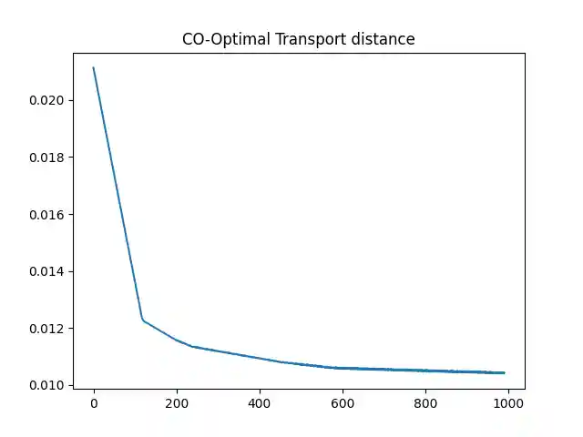
Marginal distribution = [0.07507868 0.08001347 0.09469872 0.1001999  0.10001527 0.10001687
 0.09999904 0.09979829 0.11466591 0.13551386 0.         0.
 0.         0.         0.        ]
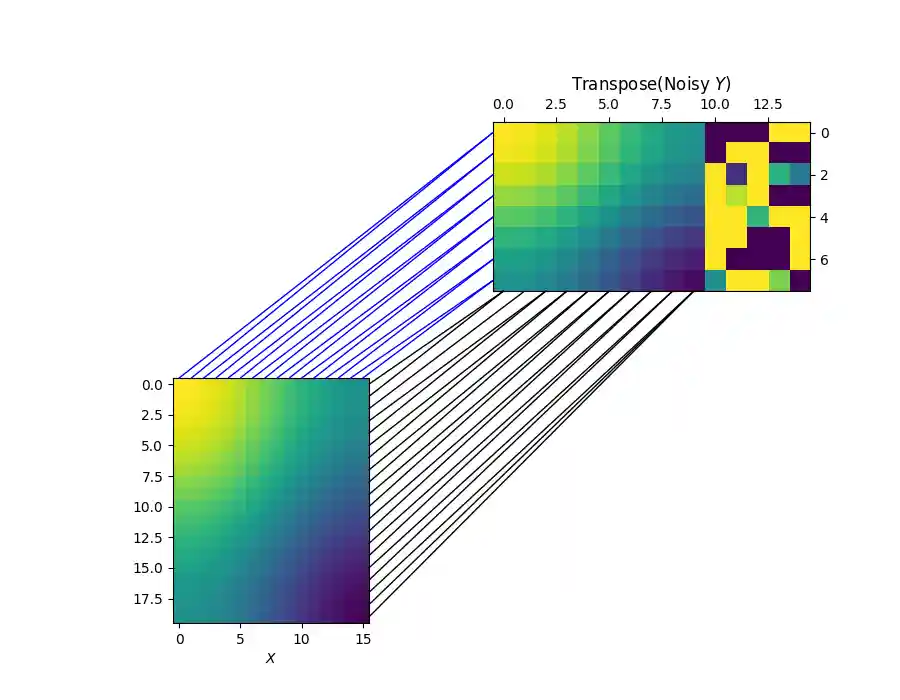
Visualizing the row and column alignments with the estimated sample marginal distribution
Clearly, the learned marginal distribution completely and successfully ignores the 5 outliers.
X, Y_noisy = X.numpy(), Y_noisy.numpy()
b = b.detach().numpy()

pi_sample, pi_feature = coot(X, Y_noisy, wy_samp=b, log=False, verbose=True)

fig = pl.figure(4, (9, 7))
pl.clf()

ax1 = pl.subplot(2, 2, 3)
pl.imshow(X, vmin=-2, vmax=2)
pl.xlabel('$X$')

ax2 = pl.subplot(2, 2, 2)
ax2.yaxis.tick_right()
pl.imshow(np.transpose(Y_noisy), vmin=-2, vmax=2)
pl.title("Transpose(Noisy $Y$)")
ax2.xaxis.tick_top()

for i in range(n1):
    j = np.argmax(pi_sample[i, :])
    xyA = (d1 - .5, i)
    xyB = (j, d2 - .5)
    con = ConnectionPatch(xyA=xyA, xyB=xyB, coordsA=ax1.transData,
                          coordsB=ax2.transData, color="black")
    fig.add_artist(con)

for i in range(d1):
    j = np.argmax(pi_feature[i, :])
    xyA = (i, -.5)
    xyB = (-.5, j)
    con = ConnectionPatch(
        xyA=xyA, xyB=xyB, coordsA=ax1.transData, coordsB=ax2.transData, color="blue")
    fig.add_artist(con)
CO-Optimal Transport cost at iteration 1: 0.010389716046318498
Total running time of the script: (0 minutes 3.856 seconds)