Smooth and sparse OT example — POT Python Optimal Transport 0.9.5 documentation
Note
Go to the end to download the full example code.
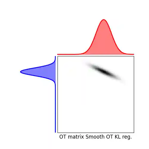
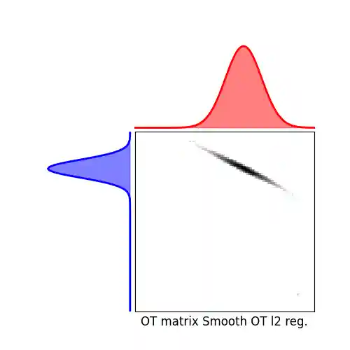
This example illustrates the computation of Smooth and Sparse (KL an L2 reg.) OT and sparsity-constrained OT, together with their visualizations.
# Author: Remi Flamary <remi.flamary@unice.fr>
#
# License: MIT License

# sphinx_gallery_thumbnail_number = 5

import numpy as np
import matplotlib.pylab as pl
import ot
import ot.plot
from ot.datasets import make_1D_gauss as gauss
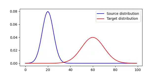
Generate data
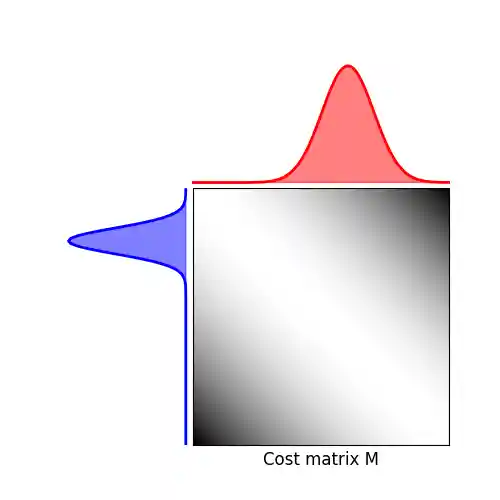
Plot distributions and loss matrix
pl.figure(1, figsize=(6.4, 3))
pl.plot(x, a, "b", label="Source distribution")
pl.plot(x, b, "r", label="Target distribution")
pl.legend()
<matplotlib.legend.Legend object at 0x7f590d7a33d0>
(<Axes: >, <Axes: >, <Axes: >)
Solve Smooth OT
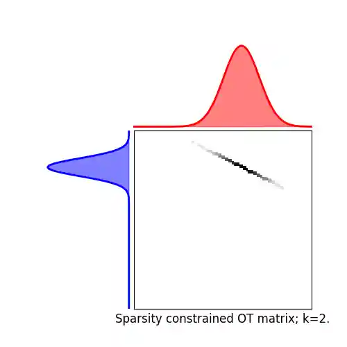
lambd = 1e-1

max_nz = 2  # two non-zero entries are permitted per column of the OT plan
Gsc = ot.smooth.smooth_ot_dual(
    a, b, M, lambd, reg_type="sparsity_constrained", max_nz=max_nz
)
pl.figure(5, figsize=(5, 5))
ot.plot.plot1D_mat(a, b, Gsc, "Sparsity constrained OT matrix; k=2.")

pl.show()
Total running time of the script: (0 minutes 0.649 seconds)