Optimal Transport with different ground metrics — POT Python Optimal Transport 0.9.6 documentation
Note
Go to the end to download the full example code.
2D OT on empirical distribution with different ground metric.
Stole the figure idea from Fig. 1 and 2 in https://arxiv.org/pdf/1706.07650.pdf
# Author: Remi Flamary <remi.flamary@unice.fr>
#
# License: MIT License

# sphinx_gallery_thumbnail_number = 3

import numpy as np
import matplotlib.pylab as pl
import ot
import ot.plot
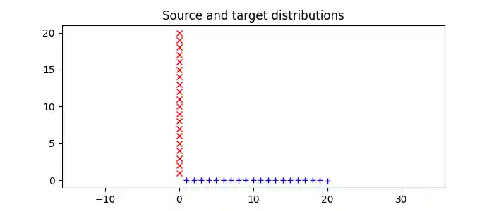
Dataset 1 : uniform sampling
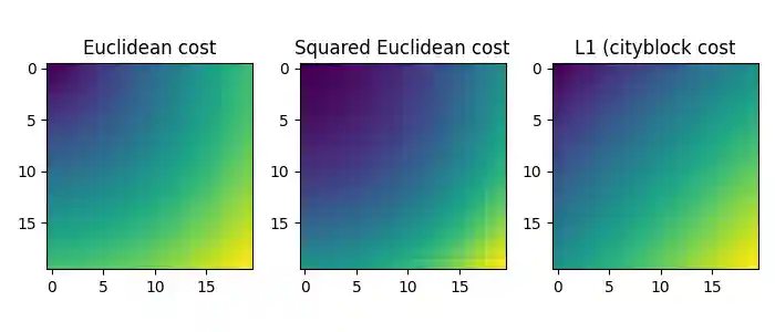
n = 20  # nb samples
xs = np.zeros((n, 2))
xs[:, 0] = np.arange(n) + 1
xs[:, 1] = (np.arange(n) + 1) * -0.001  # to make it strictly convex...

xt = np.zeros((n, 2))
xt[:, 1] = np.arange(n) + 1

a, b = ot.unif(n), ot.unif(n)  # uniform distribution on samples

# loss matrix
M1 = ot.dist(xs, xt, metric="euclidean")
M1 /= M1.max()

# loss matrix
M2 = ot.dist(xs, xt, metric="sqeuclidean")
M2 /= M2.max()

# loss matrix
Mp = ot.dist(xs, xt, metric="cityblock")
Mp /= Mp.max()

# Data
pl.figure(1, figsize=(7, 3))
pl.clf()
pl.plot(xs[:, 0], xs[:, 1], "+b", label="Source samples")
pl.plot(xt[:, 0], xt[:, 1], "xr", label="Target samples")
pl.axis("equal")
pl.title("Source and target distributions")


# Cost matrices
pl.figure(2, figsize=(7, 3))

pl.subplot(1, 3, 1)
pl.imshow(M1, interpolation="nearest")
pl.title("Euclidean cost")

pl.subplot(1, 3, 2)
pl.imshow(M2, interpolation="nearest")
pl.title("Squared Euclidean cost")

pl.subplot(1, 3, 3)
pl.imshow(Mp, interpolation="nearest")
pl.title("L1 (cityblock cost")
pl.tight_layout()
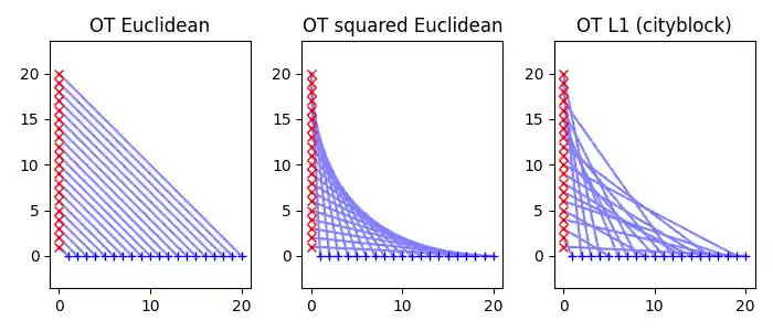
Dataset 1 : Plot OT Matrices
G1 = ot.emd(a, b, M1)
G2 = ot.emd(a, b, M2)
Gp = ot.emd(a, b, Mp)

# OT matrices
pl.figure(3, figsize=(7, 3))

pl.subplot(1, 3, 1)
ot.plot.plot2D_samples_mat(xs, xt, G1, c=[0.5, 0.5, 1])
pl.plot(xs[:, 0], xs[:, 1], "+b", label="Source samples")
pl.plot(xt[:, 0], xt[:, 1], "xr", label="Target samples")
pl.axis("equal")
# pl.legend(loc=0)
pl.title("OT Euclidean")

pl.subplot(1, 3, 2)
ot.plot.plot2D_samples_mat(xs, xt, G2, c=[0.5, 0.5, 1])
pl.plot(xs[:, 0], xs[:, 1], "+b", label="Source samples")
pl.plot(xt[:, 0], xt[:, 1], "xr", label="Target samples")
pl.axis("equal")
# pl.legend(loc=0)
pl.title("OT squared Euclidean")

pl.subplot(1, 3, 3)
ot.plot.plot2D_samples_mat(xs, xt, Gp, c=[0.5, 0.5, 1])
pl.plot(xs[:, 0], xs[:, 1], "+b", label="Source samples")
pl.plot(xt[:, 0], xt[:, 1], "xr", label="Target samples")
pl.axis("equal")
# pl.legend(loc=0)
pl.title("OT L1 (cityblock)")
pl.tight_layout()

pl.show()
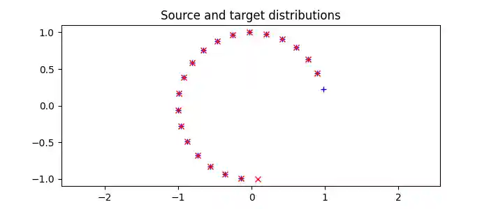
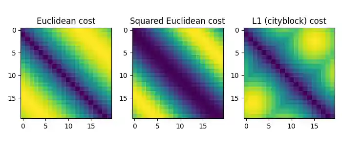
Dataset 2 : Partial circle
n = 20  # nb samples
xtot = np.zeros((n + 1, 2))
xtot[:, 0] = np.cos((np.arange(n + 1) + 1.0) * 0.8 / (n + 2) * 2 * np.pi)
xtot[:, 1] = np.sin((np.arange(n + 1) + 1.0) * 0.8 / (n + 2) * 2 * np.pi)

xs = xtot[:n, :]
xt = xtot[1:, :]

a, b = ot.unif(n), ot.unif(n)  # uniform distribution on samples

# loss matrix
M1 = ot.dist(xs, xt, metric="euclidean")
M1 /= M1.max()

# loss matrix
M2 = ot.dist(xs, xt, metric="sqeuclidean")
M2 /= M2.max()

# loss matrix
Mp = ot.dist(xs, xt, metric="cityblock")
Mp /= Mp.max()


# Data
pl.figure(4, figsize=(7, 3))
pl.clf()
pl.plot(xs[:, 0], xs[:, 1], "+b", label="Source samples")
pl.plot(xt[:, 0], xt[:, 1], "xr", label="Target samples")
pl.axis("equal")
pl.title("Source and target distributions")


# Cost matrices
pl.figure(5, figsize=(7, 3))

pl.subplot(1, 3, 1)
pl.imshow(M1, interpolation="nearest")
pl.title("Euclidean cost")

pl.subplot(1, 3, 2)
pl.imshow(M2, interpolation="nearest")
pl.title("Squared Euclidean cost")

pl.subplot(1, 3, 3)
pl.imshow(Mp, interpolation="nearest")
pl.title("L1 (cityblock) cost")
pl.tight_layout()
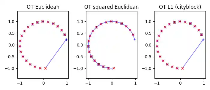
Dataset 2 : Plot OT Matrices
G1 = ot.emd(a, b, M1)
G2 = ot.emd(a, b, M2)
Gp = ot.emd(a, b, Mp)

# OT matrices
pl.figure(6, figsize=(7, 3))

pl.subplot(1, 3, 1)
ot.plot.plot2D_samples_mat(xs, xt, G1, c=[0.5, 0.5, 1])
pl.plot(xs[:, 0], xs[:, 1], "+b", label="Source samples")
pl.plot(xt[:, 0], xt[:, 1], "xr", label="Target samples")
pl.axis("equal")
# pl.legend(loc=0)
pl.title("OT Euclidean")

pl.subplot(1, 3, 2)
ot.plot.plot2D_samples_mat(xs, xt, G2, c=[0.5, 0.5, 1])
pl.plot(xs[:, 0], xs[:, 1], "+b", label="Source samples")
pl.plot(xt[:, 0], xt[:, 1], "xr", label="Target samples")
pl.axis("equal")
# pl.legend(loc=0)
pl.title("OT squared Euclidean")

pl.subplot(1, 3, 3)
ot.plot.plot2D_samples_mat(xs, xt, Gp, c=[0.5, 0.5, 1])
pl.plot(xs[:, 0], xs[:, 1], "+b", label="Source samples")
pl.plot(xt[:, 0], xt[:, 1], "xr", label="Target samples")
pl.axis("equal")
# pl.legend(loc=0)
pl.title("OT L1 (cityblock)")
pl.tight_layout()

pl.show()
Total running time of the script: (0 minutes 1.681 seconds)