Geometry of OT distances — POT Python Optimal Transport 0.9.6 documentation
Note
Go to the end to download the full example code.
Shows how to compute multiple Wasserstein and Sinkhorn with two different ground metrics and plot their values for different distributions.
# Author: Remi Flamary <remi.flamary@unice.fr>
#
# License: MIT License

# sphinx_gallery_thumbnail_number = 2

import numpy as np
import matplotlib.pylab as pl
import ot
from ot.datasets import make_1D_gauss as gauss
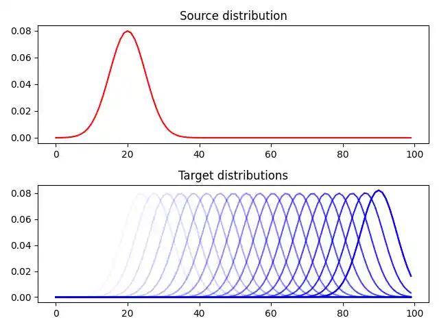
Generate data
n = 100  # nb bins
n_target = 20  # nb target distributions


# bin positions
x = np.arange(n, dtype=np.float64)

lst_m = np.linspace(20, 90, n_target)

# Gaussian distributions
a = gauss(n, m=20, s=5)  # m= mean, s= std

B = np.zeros((n, n_target))

for i, m in enumerate(lst_m):
    B[:, i] = gauss(n, m=m, s=5)

# loss matrix and normalization
M = ot.dist(x.reshape((n, 1)), x.reshape((n, 1)), "euclidean")
M /= M.max() * 0.1
M2 = ot.dist(x.reshape((n, 1)), x.reshape((n, 1)), "sqeuclidean")
M2 /= M2.max() * 0.1
Plot data
pl.figure(1)
pl.subplot(2, 1, 1)
pl.plot(x, a, "r", label="Source distribution")
pl.title("Source distribution")
pl.subplot(2, 1, 2)
for i in range(n_target):
    pl.plot(x, B[:, i], "b", alpha=i / n_target)
pl.plot(x, B[:, -1], "b", label="Target distributions")
pl.title("Target distributions")
pl.tight_layout()
Compute EMD for the different losses
d_emd = ot.emd2(a, B, M)  # direct computation of OT loss
d_emd2 = ot.emd2(a, B, M2)  # direct computation of OT loss with metric M2
d_tv = [np.sum(abs(a - B[:, i])) for i in range(n_target)]

pl.figure(2)
pl.subplot(2, 1, 1)
pl.plot(x, a, "r", label="Source distribution")
pl.title("Distributions")
for i in range(n_target):
    pl.plot(x, B[:, i], "b", alpha=i / n_target)
pl.plot(x, B[:, -1], "b", label="Target distributions")
pl.ylim((-0.01, 0.13))
pl.xticks(())
pl.legend()
pl.subplot(2, 1, 2)
pl.plot(d_emd, label="Euclidean OT")
pl.plot(d_emd2, label="Squared Euclidean OT")
pl.plot(d_tv, label="Total Variation (TV)")
# pl.xlim((-7,23))
pl.xlabel("Displacement")
pl.title("Divergences")
pl.legend()
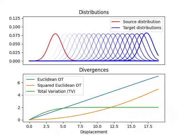
<matplotlib.legend.Legend object at 0x7f95b53558d0>
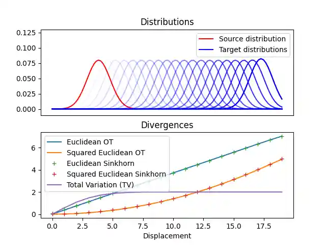
Compute Sinkhorn for the different losses
reg = 1e-1
d_sinkhorn = ot.sinkhorn2(a, B, M, reg)
d_sinkhorn2 = ot.sinkhorn2(a, B, M2, reg)

pl.figure(3)
pl.clf()

pl.subplot(2, 1, 1)
pl.plot(x, a, "r", label="Source distribution")
pl.title("Distributions")
for i in range(n_target):
    pl.plot(x, B[:, i], "b", alpha=i / n_target)
pl.plot(x, B[:, -1], "b", label="Target distributions")
pl.ylim((-0.01, 0.13))
pl.xticks(())
pl.legend()
pl.subplot(2, 1, 2)
pl.plot(d_emd, label="Euclidean OT")
pl.plot(d_emd2, label="Squared Euclidean OT")
pl.plot(d_sinkhorn, "+", label="Euclidean Sinkhorn")
pl.plot(d_sinkhorn2, "+", label="Squared Euclidean Sinkhorn")
pl.plot(d_tv, label="Total Variation (TV)")
# pl.xlim((-7,23))
pl.xlabel("Displacement")
pl.title("Divergences")
pl.legend()
pl.show()
Total running time of the script: (0 minutes 0.778 seconds)