Sliced Wasserstein Distance on 2D distributions — POT Python Optimal Transport 0.9.6 documentation
Note
Go to the end to download the full example code.
Note
Example added in release: 0.8.0.
This example illustrates the computation of the sliced Wasserstein Distance as proposed in [31].
[31] Bonneel, Nicolas, et al. “Sliced and radon wasserstein barycenters of measures.” Journal of Mathematical Imaging and Vision 51.1 (2015): 22-45
# Author: Adrien Corenflos <adrien.corenflos@aalto.fi>
#
# License: MIT License

# sphinx_gallery_thumbnail_number = 2

import matplotlib.pylab as pl
import numpy as np

import ot
Generate data
n = 200  # nb samples

mu_s = np.array([0, 0])
cov_s = np.array([[1, 0], [0, 1]])

mu_t = np.array([4, 4])
cov_t = np.array([[1, -0.8], [-0.8, 1]])

xs = ot.datasets.make_2D_samples_gauss(n, mu_s, cov_s)
xt = ot.datasets.make_2D_samples_gauss(n, mu_t, cov_t)

a, b = np.ones((n,)) / n, np.ones((n,)) / n  # uniform distribution on samples
Plot data
pl.figure(1)
pl.plot(xs[:, 0], xs[:, 1], "+b", label="Source samples")
pl.plot(xt[:, 0], xt[:, 1], "xr", label="Target samples")
pl.legend(loc=0)
pl.title("Source and target distributions")
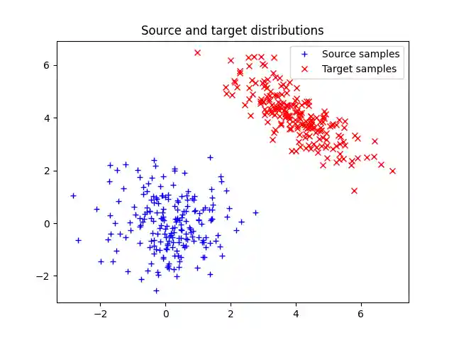
Text(0.5, 1.0, 'Source and target distributions')
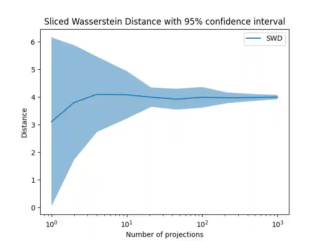
Sliced Wasserstein distance for different seeds and number of projections
Plot Sliced Wasserstein Distance
Total running time of the script: (0 minutes 2.410 seconds)