Spherical Sliced Wasserstein on distributions in S^2 — POT Python Optimal Transport 0.9.6 documentation
Note
Go to the end to download the full example code.
Note
Example added in release: 0.8.0.
This example illustrates the computation of the spherical sliced Wasserstein discrepancy as proposed in [46].
[46] Bonet, C., Berg, P., Courty, N., Septier, F., Drumetz, L., & Pham, M. T. (2023). ‘Spherical Sliced-Wasserstein”. International Conference on Learning Representations.
# Author: Clément Bonet <clement.bonet@univ-ubs.fr>
#
# License: MIT License

# sphinx_gallery_thumbnail_number = 1

import matplotlib.pylab as pl
import numpy as np

import ot
Generate data
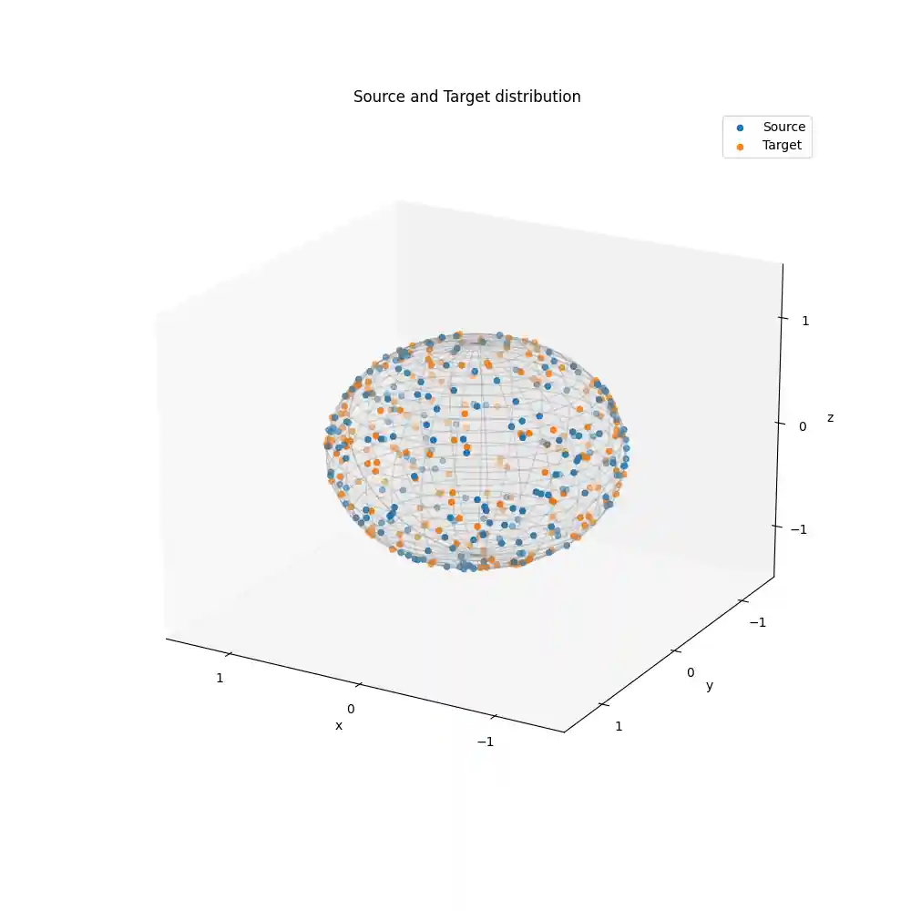
Plot data
fig = pl.figure(figsize=(10, 10))
ax = pl.axes(projection="3d")
ax.grid(False)

u, v = np.mgrid[0 : 2 * np.pi : 30j, 0 : np.pi : 30j]
x = np.cos(u) * np.sin(v)
y = np.sin(u) * np.sin(v)
z = np.cos(v)
ax.plot_surface(x, y, z, color="gray", alpha=0.03)
ax.plot_wireframe(x, y, z, linewidth=1, alpha=0.25, color="gray")

ax.scatter(xs[:, 0], xs[:, 1], xs[:, 2], label="Source")
ax.scatter(xt[:, 0], xt[:, 1], xt[:, 2], label="Target")

fs = 10
# Labels
ax.set_xlabel("x", fontsize=fs)
ax.set_ylabel("y", fontsize=fs)
ax.set_zlabel("z", fontsize=fs)

ax.view_init(20, 120)
ax.set_xlim(-1.5, 1.5)
ax.set_ylim(-1.5, 1.5)
ax.set_zlim(-1.5, 1.5)

# Ticks
ax.set_xticks([-1, 0, 1])
ax.set_yticks([-1, 0, 1])
ax.set_zticks([-1, 0, 1])

pl.legend(loc=0)
pl.title("Source and Target distribution")
Text(0.5, 1.0, 'Source and Target distribution')
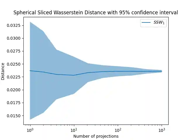
Spherical Sliced Wasserstein for different seeds and number of projections
Plot Spherical Sliced Wasserstein
Total running time of the script: (0 minutes 56.334 seconds)