1D Unbalanced optimal transport — POT Python Optimal Transport 0.9.6 documentation
Note
Go to the end to download the full example code.
This example illustrates the computation of Unbalanced Optimal transport using a Kullback-Leibler relaxation.
# Author: Hicham Janati <hicham.janati@inria.fr>
#
# License: MIT License

# sphinx_gallery_thumbnail_number = 4

import numpy as np
import matplotlib.pylab as pl
import ot
import ot.plot
from ot.datasets import make_1D_gauss as gauss
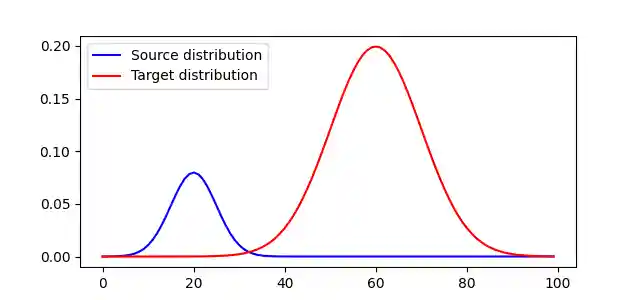
Generate data
Plot distributions and loss matrix
pl.figure(1, figsize=(6.4, 3))
pl.plot(x, a, "b", label="Source distribution")
pl.plot(x, b, "r", label="Target distribution")
pl.legend()

# plot distributions and loss matrix

pl.figure(2, figsize=(5, 5))
ot.plot.plot1D_mat(a, b, M, "Cost matrix M")
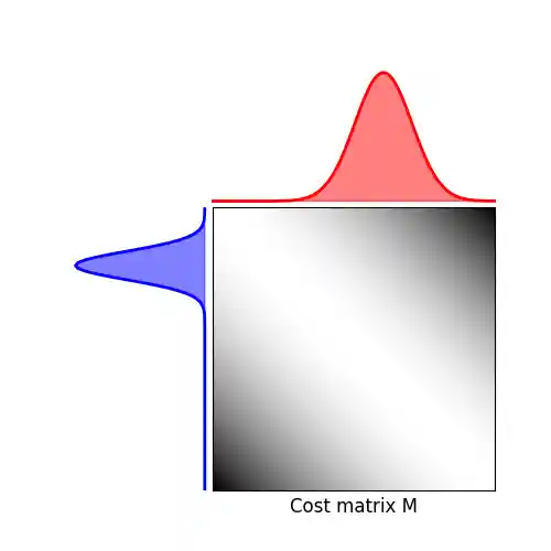
(<Axes: >, <Axes: >, <Axes: >)
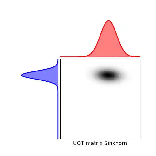
Solve Unbalanced Sinkhorn
# Sinkhorn

epsilon = 0.1  # entropy parameter
alpha = 1.0  # Unbalanced KL relaxation parameter
Gs = ot.unbalanced.sinkhorn_unbalanced(a, b, M, epsilon, alpha, verbose=True)

pl.figure(3, figsize=(5, 5))
ot.plot.plot1D_mat(a, b, Gs, "UOT matrix Sinkhorn")

pl.show()
plot the transported mass
pl.figure(4, figsize=(6.4, 3))
pl.plot(x, a, "b", label="Source distribution")
pl.plot(x, b, "r", label="Target distribution")
pl.fill(x, Gs.sum(1), "b", alpha=0.5, label="Transported source")
pl.fill(x, Gs.sum(0), "r", alpha=0.5, label="Transported target")
pl.legend(loc="upper right")
pl.title("Distributions and transported mass for UOT")
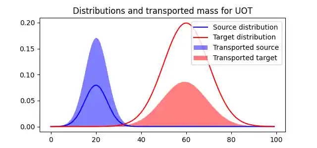
Text(0.5, 1.0, 'Distributions and transported mass for UOT')
Total running time of the script: (0 minutes 0.283 seconds)