Smooth and sparse OT example — POT Python Optimal Transport 0.9.6dev0 documentation
Note
Go to the end to download the full example code.
Note
Example updated in release: 0.9.1.
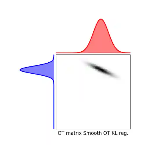
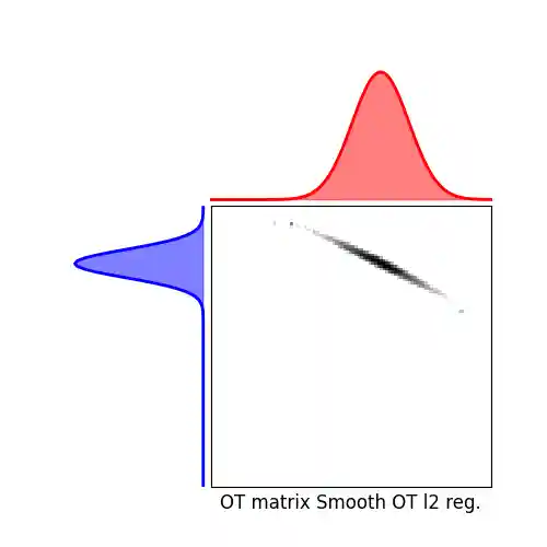
This example illustrates the computation of Smooth and Sparse (KL an L2 reg.) OT and sparsity-constrained OT, together with their visualizations.
# Author: Remi Flamary <remi.flamary@unice.fr>
#
# License: MIT License

# sphinx_gallery_thumbnail_number = 5

import numpy as np
import matplotlib.pylab as pl
import ot
import ot.plot
from ot.datasets import make_1D_gauss as gauss
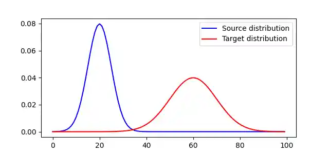
Generate data
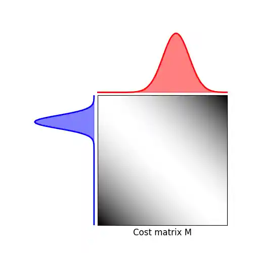
Plot distributions and loss matrix
pl.figure(1, figsize=(6.4, 3))
pl.plot(x, a, "b", label="Source distribution")
pl.plot(x, b, "r", label="Target distribution")
pl.legend()
<matplotlib.legend.Legend object at 0x7f6f3558cdc0>
(<Axes: >, <Axes: >, <Axes: >)
Solve Smooth OT
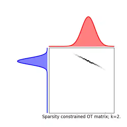
lambd = 1e-1

max_nz = 2  # two non-zero entries are permitted per column of the OT plan
Gsc = ot.smooth.smooth_ot_dual(
    a, b, M, lambd, reg_type="sparsity_constrained", max_nz=max_nz
)
pl.figure(5, figsize=(5, 5))
ot.plot.plot1D_mat(a, b, Gsc, "Sparsity constrained OT matrix; k=2.")

pl.show()
Total running time of the script: (0 minutes 1.354 seconds)