Sliced Unbalanced optimal transport — POT Python Optimal Transport 0.9.7.dev0 documentation
Note
Go to the end to download the full example code.
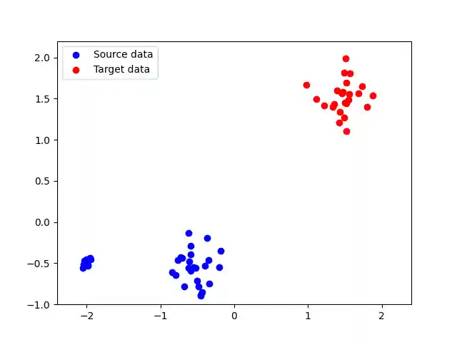
This example illustrates the behavior of Sliced UOT versus Unbalanced Sliced OT, introduced in [82]. The first one removes outliers on each slice while the second one removes outliers of the original marginals.
[82] Bonet, C., Nadjahi, K., Séjourné, T., Fatras, K., & Courty, N. (2025). Slicing Unbalanced Optimal Transport. Transactions on Machine Learning Research.
# Author: Clément Bonet <clement.bonet.mapp@polytechnique.edu>
#         Nicolas Courty <nicolas.courty@irisa.fr>
#
# License: MIT License

# sphinx_gallery_thumbnail_number = 4

import numpy as np
import matplotlib.pylab as pl
import ot
import torch
import matplotlib.pyplot as plt
import matplotlib.animation as animation

from sklearn.neighbors import KernelDensity
Generate data
np.random.seed(42)

n_samples = 25  # 500
nb_outliers = 10  # 200


mu_s = np.array([0, 0]) - 0.5
cov_s = 0.2**2 * np.array([[1, 0], [0, 1]])

mu_s_outliers = -np.array([2, 0.5])
cov_s_outliers = 0.05**2 * np.array([[1, 0], [0, 1]])

mu_t = np.array([0, 0]) + 1.5
cov_t = 0.2**2 * np.array([[1, 0], [0, 1]])


def generate_dataset(n_samples):
    # Generate source data (with outliers)
    Xs = ot.datasets.make_2D_samples_gauss(n_samples, mu_s, cov_s)
    Xs_outlier = ot.datasets.make_2D_samples_gauss(
        nb_outliers, mu_s_outliers, cov_s_outliers
    )

    Xs = np.vstack((Xs, Xs_outlier))
    Xs_torch = torch.from_numpy(Xs).type(torch.float)

    # Generate target data
    Xt = ot.datasets.make_2D_samples_gauss(n_samples, mu_t, cov_t)
    Xt_torch = torch.from_numpy(Xt).type(torch.float)

    return Xs_torch, Xt_torch


Xs, Xt = generate_dataset(n_samples)

pl.figure(1)
pl.scatter(Xs[:, 0], Xs[:, 1], color="blue", label="Source data")
pl.scatter(Xt[:, 0], Xt[:, 1], color="red", label="Target data")
pl.xlim(-2.4, 2.4)
pl.ylim(-1, 2.2)
pl.legend()
pl.show()
Compute SUOT and USOT
p = 2
num_proj = 180

a = torch.ones(Xs.shape[0], dtype=torch.float)
b = torch.ones(Xt.shape[0], dtype=torch.float)

# construct projections
thetas = np.linspace(0, np.pi, num_proj)
dir = np.array([(np.cos(theta), np.sin(theta)) for theta in thetas])
dir_torch = torch.from_numpy(dir).type(torch.float)

# Coordinates of the projections
Xps = (Xs @ dir_torch.T).T  # shape (n_projs, n)
Xpt = (Xt @ dir_torch.T).T

# Projections on the lines
projs_Xps = Xps[:, :, None] * dir_torch[:, None, :]  # shape (n_projs, n, p)
projs_Xpt = Xpt[:, :, None] * dir_torch[:, None, :]


# Compute SUOT
rho1_SUOT = 1
rho2_SUOT = 1

_, log = ot.unbalanced.sliced_unbalanced_ot(
    Xs,
    Xt,
    (rho1_SUOT, rho2_SUOT),
    a,
    b,
    num_proj,
    p,
    numItermax=10,
    projections=dir_torch.T,
    log=True,
)
A_SUOT, B_SUOT = log["a_reweighted"].T, log["b_reweighted"].T


# Compute USOT
rho1_USOT = 1
rho2_USOT = 1

A_USOT, B_USOT, _ = ot.unbalanced_sliced_ot(
    Xs,
    Xt,
    (rho1_USOT, rho2_USOT),
    a,
    b,
    num_proj,
    p,
    numItermax=10,
    projections=dir_torch.T,
)
Sliced Unbalanced OT
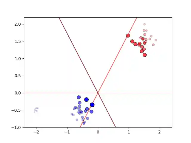
SUOT averages UOT problems on different slices. Depending on the slice, SUOT can keep or get rid of the outlier mode.
get_rot = lambda theta: np.array(
    [[np.cos(theta), -np.sin(theta)], [np.sin(theta), np.cos(theta)]]
)

# visu parameters
nb_slices = 180  # 60
offset_degree = int(180 / nb_slices)

delta_degree = np.pi / nb_slices
colors = plt.cm.Reds(np.linspace(0.3, 1, nb_slices))

X1 = np.array([-4, 0])
X2 = np.array([4, 0])

# max_weights = max(A_SUOT.max(), B_SUOT.max())


pl.figure(1)


def _update_plot(i):
    weights_src = A_SUOT[i * offset_degree, :].cpu().numpy()
    weights_tgt = B_SUOT[i * offset_degree, :].cpu().numpy()

    max_weights = max(weights_src.max(), weights_tgt.max())
    min_weights = min(weights_src.min(), weights_tgt.min())

    weights_src = 0.1 + 0.9 * (weights_src - min_weights) / (max_weights - min_weights)
    weights_tgt = 0.1 + 0.9 * (weights_tgt - min_weights) / (max_weights - min_weights)

    R = get_rot(delta_degree * (-i))

    X1_r = X1.dot(R)
    X2_r = X2.dot(R)

    pl.clf()

    pl.plot(
        [X1_r[0], X2_r[0]], [X1_r[1], X2_r[1]], color=colors[i], alpha=0.8, zorder=0
    )

    for j in range(len(Xs)):
        pl.plot(
            [Xs[j, 0], projs_Xps[i * offset_degree, j, 0]],
            [Xs[j, 1], projs_Xps[i * offset_degree, j, 1]],
            c="blue",
            alpha=weights_src[j],
        )

    for j in range(len(Xt)):
        pl.plot(
            [Xt[j, 0], projs_Xpt[i * offset_degree, j, 0]],
            [Xt[j, 1], projs_Xpt[i * offset_degree, j, 1]],
            c="red",
            alpha=weights_tgt[j],
        )

    pl.scatter(
        Xs[:, 0],
        Xs[:, 1],
        s=100 * weights_src,
        alpha=weights_src,
        zorder=1,
        color="blue",
        label="Source data",
        edgecolor="black",
    )
    pl.scatter(
        Xt[:, 0],
        Xt[:, 1],
        s=100 * weights_tgt,
        alpha=weights_tgt,
        zorder=1,
        color="red",
        label="Target data",
        edgecolors="black",
    )

    pl.xlim(-2.4, 2.4)
    pl.ylim(-1, 2.2)

    return 1


weights_src = A_SUOT[0, :].cpu().numpy()
weights_tgt = B_SUOT[0, :].cpu().numpy()

max_weights = max(weights_src.max(), weights_tgt.max())
min_weights = min(weights_src.min(), weights_tgt.min())

weights_src = 0.1 + 0.9 * (weights_src - min_weights) / (max_weights - min_weights)
weights_tgt = 0.1 + 0.9 * (weights_tgt - min_weights) / (max_weights - min_weights)

X1_r, X2_r = X1, X2

pl.plot(
    [X1_r[0], X2_r[0]],
    [X1_r[1], X2_r[1]],
    color=colors[0],
    alpha=0.8,
    zorder=0,
    label="Directions",
)

for j in range(len(Xs)):
    pl.plot(
        [Xs[j, 0], projs_Xps[0, j, 0]],
        [Xs[j, 1], projs_Xps[0, j, 1]],
        c="blue",
        alpha=weights_src[j],
    )

for j in range(len(Xt)):
    pl.plot(
        [Xt[j, 0], projs_Xpt[0, j, 0]],
        [Xt[j, 1], projs_Xpt[0, j, 1]],
        c="red",
        alpha=weights_tgt[j],
    )

pl.scatter(
    Xs[:, 0],
    Xs[:, 1],
    s=100 * weights_src,
    alpha=weights_src,
    zorder=1,
    color="blue",
    label="Source data",
    edgecolor="black",
)
pl.scatter(
    Xt[:, 0],
    Xt[:, 1],
    s=100 * weights_tgt,
    alpha=weights_tgt,
    zorder=1,
    color="red",
    label="Target data",
    edgecolors="black",
)

pl.xlim(-2.4, 2.4)
pl.ylim(-1, 2.2)

ani = animation.FuncAnimation(
    pl.gcf(),
    _update_plot,
    nb_slices,
    interval=100,  # , repeat_delay=2000
)
Unbalanced Sliced OT
USOT is able to get rid of the outlier mode on all slices, as it reweights the original distributions.
# visu parameters
nb_slices = 3
offset_degree = int(180 / nb_slices)

delta_degree = np.pi / nb_slices
colors = plt.cm.Reds(np.linspace(0.3, 1, nb_slices))

plt.figure(1)

for i in range(nb_slices):
    weights_src = A_USOT.cpu().numpy()
    weights_tgt = B_USOT.cpu().numpy()

    max_weights = max(weights_src.max(), weights_tgt.max())
    min_weights = min(weights_src.min(), weights_tgt.min())

    weights_src = 0.1 + 0.9 * (weights_src - min_weights) / (max_weights - min_weights)
    weights_tgt = 0.1 + 0.9 * (weights_tgt - min_weights) / (max_weights - min_weights)

    R = get_rot(delta_degree * (-i))
    X1_r = X1.dot(R)
    X2_r = X2.dot(R)
    if i == 0:
        pl.plot(
            [X1_r[0], X2_r[0]],
            [X1_r[1], X2_r[1]],
            color=colors[i],
            alpha=0.8,
            zorder=0,
            label="Directions",
        )
    else:
        pl.plot(
            [X1_r[0], X2_r[0]], [X1_r[1], X2_r[1]], color=colors[i], alpha=0.8, zorder=0
        )

pl.scatter(
    Xs[:, 0],
    Xs[:, 1],
    s=100 * weights_src,
    alpha=weights_src,
    zorder=1,
    color="blue",
    label="Source data",
    edgecolors="black",
)
pl.scatter(
    Xt[:, 0],
    Xt[:, 1],
    s=100 * weights_tgt,
    alpha=weights_tgt,
    zorder=1,
    color="red",
    label="Target data",
    edgecolors="black",
)
pl.xlim(-2.4, 2.4)
pl.ylim(-1, 2.2)
pl.show()
Utils plot
def kde_sklearn(x, x_grid, weights=None, bandwidth=0.2, **kwargs):
    """Kernel Density Estimation with Scikit-learn"""
    kde_skl = KernelDensity(bandwidth=bandwidth, **kwargs)
    if weights is not None:
        kde_skl.fit(x[:, np.newaxis], sample_weight=weights)
    else:
        kde_skl.fit(x[:, np.newaxis])
    # score_samples() returns the log-likelihood of the samples
    log_pdf = kde_skl.score_samples(x_grid[:, np.newaxis])
    return np.exp(log_pdf)


def plot_slices(
    col,
    nb_slices,
    x_grid,
    Xps,
    Xpt,
    Xps_weights,
    Xpt_weights,
    method,
    rho1,
    rho2,
    offset_degree,
    bw=0.05,
):
    """
    Plot the density (using a kernel estimator) of the projections on each of the slices.

    Parameters
    ----------
    col: int
        Column of the subplot
    nb_slices: int
        Number of slices on which we project
    x_grid: numpy array
        Grid of the x-abscisse
    Xps: array-like of shape (nb_slices, n_points)
        Projections of the 1st marginal in 1D
    Xpt: array-like of shape (nb_slices, m_points)
        Projections of the 2nd marginal in 1D
    Xps_weights: array_like of shape (nb_slices, n_points)
        Weights of the projections Xps
    Xpt_weights: array_like of shape (nb_slices, m_points)
        Weights of the projections Xpt
    method: str
        Legend
    rho1: int
        Legend
    rho2: int
        Legend
    offset_degree: int
    bw: float
        Bandwidth for the KDE estimation
    """
    for i in range(nb_slices):
        ax = plt.subplot2grid((nb_slices, 3), (i, col))
        if len(Xps_weights.shape) > 1:  # SUOT
            weights_src = Xps_weights[i * offset_degree, :].cpu().numpy()
            weights_tgt = Xpt_weights[i * offset_degree, :].cpu().numpy()
        else:  # USOT
            weights_src = Xps_weights.cpu().numpy()
            weights_tgt = Xpt_weights.cpu().numpy()

        samples_src = Xps[i * offset_degree, :].cpu().numpy()
        samples_tgt = Xpt[i * offset_degree, :].cpu().numpy()

        pdf_source = kde_sklearn(samples_src, x_grid, weights=weights_src, bandwidth=bw)
        pdf_target = kde_sklearn(samples_tgt, x_grid, weights=weights_tgt, bandwidth=bw)
        pdf_source_without_w = kde_sklearn(samples_src, x_grid, bandwidth=bw)
        pdf_target_without_w = kde_sklearn(samples_tgt, x_grid, bandwidth=bw)

        ax.plot(x_grid, pdf_source, color="blue", alpha=0.8, lw=2)
        ax.fill(x_grid, pdf_source_without_w, ec="grey", fc="grey", alpha=0.3)
        ax.fill(x_grid, pdf_source, ec="blue", fc="blue", alpha=0.3)

        ax.plot(x_grid, pdf_target, color="red", alpha=0.8, lw=2)
        ax.fill(x_grid, pdf_target_without_w, ec="grey", fc="grey", alpha=0.3)
        ax.fill(x_grid, pdf_target, ec="blue", fc="red", alpha=0.3)

        ax.set_xlim(xlim_min, xlim_max)

        if col == 1:
            ax.set_ylabel(
                r"$\theta=${}$^o$".format(i * offset_degree),
                color=colors[i],
                fontsize=13,
            )

        ax.set_yticks([])
        ax.set_xticks([])

        ax.set_xlabel(
            r"{}  $\rho_1={}$ $\rho_2={}$".format(method, rho1, rho2), fontsize=13
        )
Plot reweighted distributions on several slices
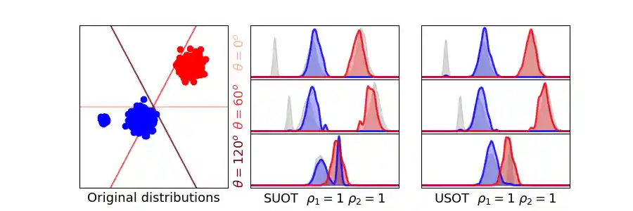
We plot the reweighted distributions on several slices (replicating Figure 1 of [82]). We see that for SUOT, the mode of outliers is kept of some slices (e.g. for \(\theta=120°\)) while USOT is able to get rid of the outlier mode.
get_rot = lambda theta: np.array(
    [[np.cos(theta), -np.sin(theta)], [np.sin(theta), np.cos(theta)]]
)

n_samples = 500
nb_outliers = 200

Xs, Xt = generate_dataset(n_samples)

Xps = (Xs @ dir_torch.T).T  # shape (n_projs, n)
Xpt = (Xt @ dir_torch.T).T

a = torch.ones(Xs.shape[0], dtype=torch.float)
b = torch.ones(Xt.shape[0], dtype=torch.float)

rho1_SUOT = 1
rho2_SUOT = 1

_, log = ot.unbalanced.sliced_unbalanced_ot(
    Xs,
    Xt,
    (rho1_SUOT, rho2_SUOT),
    a,
    b,
    num_proj,
    p,
    numItermax=10,
    projections=dir_torch.T,
    log=True,
)
A_SUOT, B_SUOT = log["a_reweighted"].T, log["b_reweighted"].T


rho1_USOT = 1
rho2_USOT = 1

A_USOT, B_USOT, _ = ot.unbalanced_sliced_ot(
    Xs,
    Xt,
    (rho1_USOT, rho2_USOT),
    a,
    b,
    num_proj,
    p,
    numItermax=10,
    projections=dir_torch.T,
)


# define plotting grid
xlim_min = -3
xlim_max = 3
x_grid = np.linspace(xlim_min, xlim_max, 200)

# visu parameters
nb_slices = 3
offset_degree = int(180 / nb_slices)

delta_degree = np.pi / nb_slices
colors = plt.cm.Reds(np.linspace(0.3, 1, nb_slices))

X1 = np.array([-4, 0])
X2 = np.array([4, 0])

fig = plt.figure(figsize=(9, 3))

ax1 = plt.subplot2grid((nb_slices, 3), (0, 0), rowspan=nb_slices)

for i in range(nb_slices):
    R = get_rot(delta_degree * (-i))
    X1_r = X1.dot(R)
    X2_r = X2.dot(R)
    if i == 0:
        ax1.plot(
            [X1_r[0], X2_r[0]],
            [X1_r[1], X2_r[1]],
            color=colors[i],
            alpha=0.8,
            zorder=0,
            label="Directions",
        )
    else:
        ax1.plot(
            [X1_r[0], X2_r[0]], [X1_r[1], X2_r[1]], color=colors[i], alpha=0.8, zorder=0
        )

ax1.scatter(Xs[:, 0], Xs[:, 1], zorder=1, color="blue", label="Source data")
ax1.scatter(Xt[:, 0], Xt[:, 1], zorder=1, color="red", label="Target data")
ax1.set_xlim([-3, 3])
ax1.set_ylim([-3, 3])
ax1.set_yticks([])
ax1.set_xticks([])
# ax1.legend(loc='best',fontsize=13)
ax1.set_xlabel("Original distributions", fontsize=13)


fig.subplots_adjust(hspace=0)
fig.subplots_adjust(wspace=0.15)

plot_slices(
    1,
    nb_slices,
    x_grid,
    Xps,
    Xpt,
    A_SUOT,
    B_SUOT,
    "SUOT",
    rho1_SUOT,
    rho2_SUOT,
    offset_degree,
)
plot_slices(
    2,
    nb_slices,
    x_grid,
    Xps,
    Xpt,
    A_USOT,
    B_USOT,
    "USOT",
    rho1_USOT,
    rho2_USOT,
    offset_degree,
)

plt.show()
Total running time of the script: (1 minutes 15.570 seconds)