The cylindrical and polar stereographic projections are detailed separately in cylindrical plots and polar plots.
Example 31: UKCP projection#
Plotting using the UKCP projection#
f = cf.read(f"cfplot_data/ukcp_rcm_test.nc")[0]

cfp.mapset(proj="UKCP", resolution="50m")
cfp.levs(-3, 7, 0.5)
cfp.setvars(grid_x_spacing=1, grid_y_spacing=1)

cfp.con(f, lines=False)
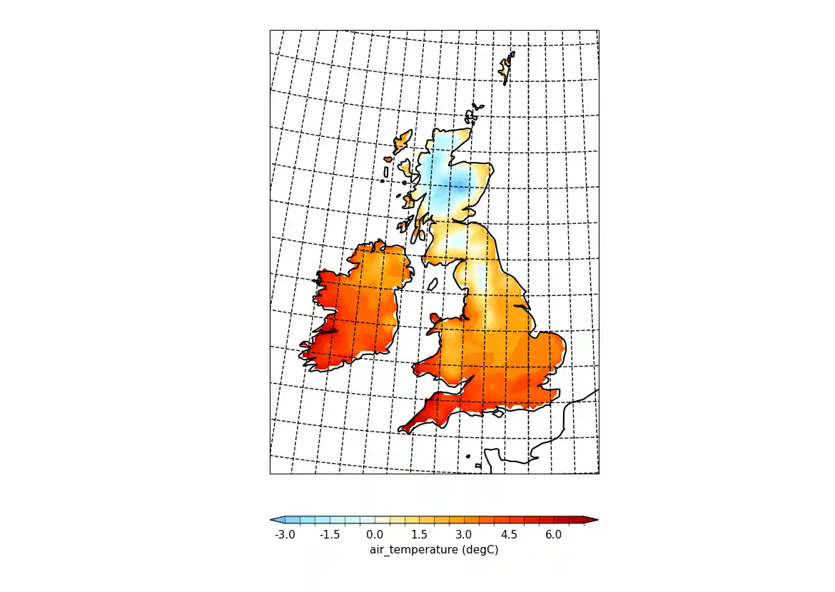
cf-plot looks for auxiliary coordinates of longitude and latitude and uses them if found. If they aren't present then cf-plot will generate the grid required using the projection_x_coordinate and projection_y_coordinate variables.
For a blockfill plot it uses the latter method and the supplied bounds.
Example 32: UKCP projection with blockfill#
Plotting a blockfill plot using the UKCP projection#
f = cf.read(f"cfplot_data/ukcp_rcm_test.nc")[0]

cfp.mapset(proj="UKCP", resolution="50m")
cfp.levs(-3, 7, 0.5)
cfp.setvars(grid_colour="grey")

cfp.con(
    f,
    lines=False,
    blockfill=True,
    # Centered over UK region with spacing of 1 each
    xticks=np.arange(14) - 11,
    yticks=np.arange(13) + 49,
)

cfp.setvars options affecting the grid plotting for the UKCP grid are:
grid=True - draw grid
grid_spacing=1 - grid spacing in degrees
grid_colour='black' - grid colour
grid_linestyle='--' - grid line style
grid_thickness=1.0 - grid thickness
Here we changed the plotted grid with the grid_colour option to cfp.setvars, xticks and yticks options to cfp.con and make a blockfill plot.
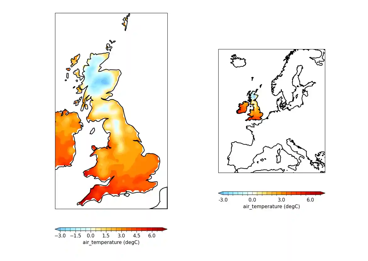
Example 33: OSGB and EuroPP projections#
Plotting using the projections OSGB and EuroPP#
f = cf.read(f"cfplot_data/ukcp_rcm_test.nc")[0]

cfp.levs(-3, 7, 0.5)

cfp.gopen(columns=2)
cfp.mapset(proj="OSGB", resolution="50m")
cfp.con(f, lines=False, colorbar_label_skip=2)
cfp.gpos(2)
cfp.mapset(proj="EuroPP", resolution="50m")
cfp.con(f, lines=False, colorbar_label_skip=2)
cfp.gclose()
Example 34: Cropping the Lambert Conformal Conic (LCC) projection#
Plotting using the Lambert Conformal Conic (LCC) projection and cropping the displayed boundaries.#
f = cf.read(f"cfplot_data/tas_A1.nc")[0]

cfp.mapset(proj="lcc", lonmin=-50, lonmax=50, latmin=20, latmax=85)

cfp.con(f.subspace(time=15))
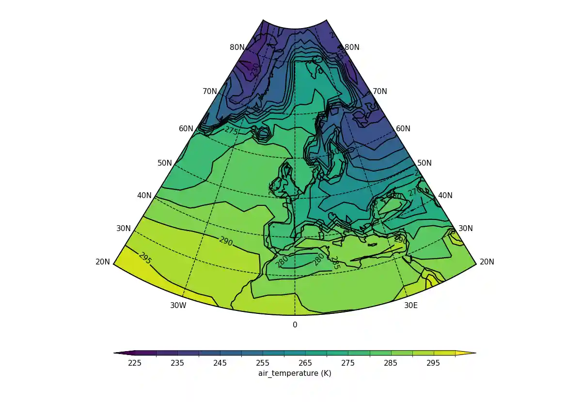
Lambert conformal projections can be cropped.
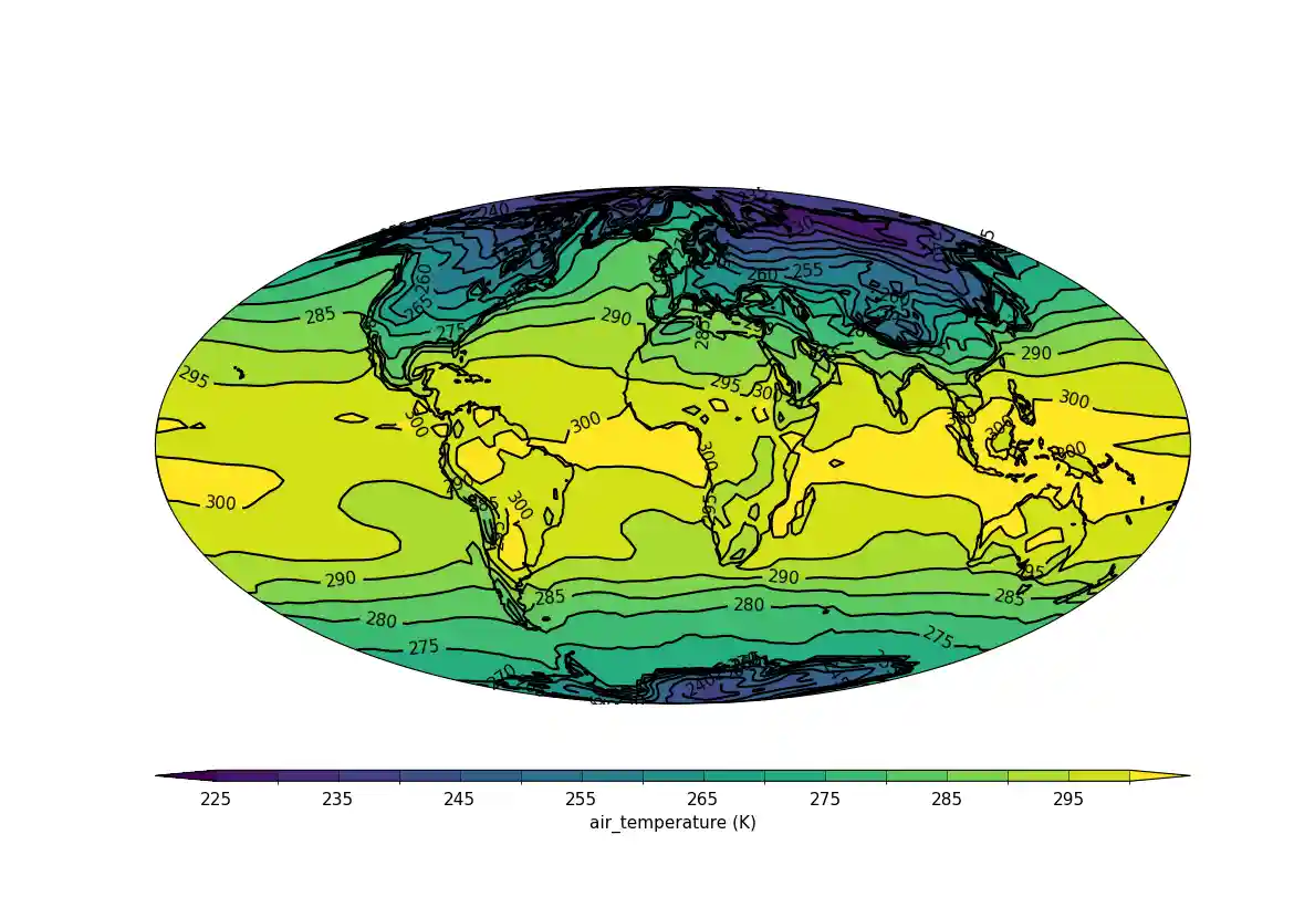
Example 35: Mollweide projection#
Plotting using the Mollweide projection#
f = cf.read(f"cfplot_data/tas_A1.nc")[0]

cfp.mapset(proj="moll")

cfp.con(f.subspace(time=15))
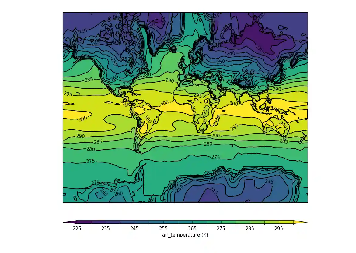
Example 36: Mercator projection#
Plotting using the Mercator projection#
f = cf.read(f"cfplot_data/tas_A1.nc")[0]

cfp.mapset(proj="merc")

cfp.con(f.subspace(time=15))
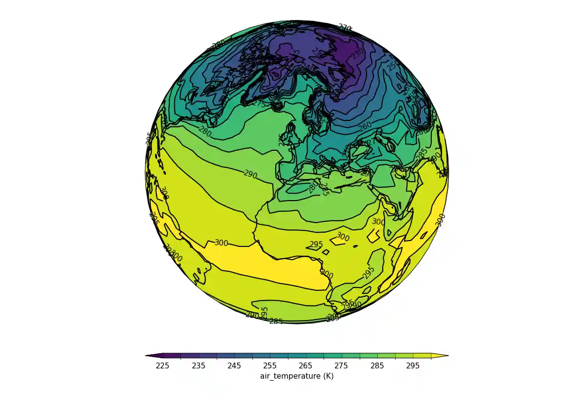
Example 37: Orthographic projection#
Plotting using the Orthographic projection#
f = cf.read(f"cfplot_data/tas_A1.nc")[0]

cfp.mapset(proj="ortho")

cfp.con(f.subspace(time=15))
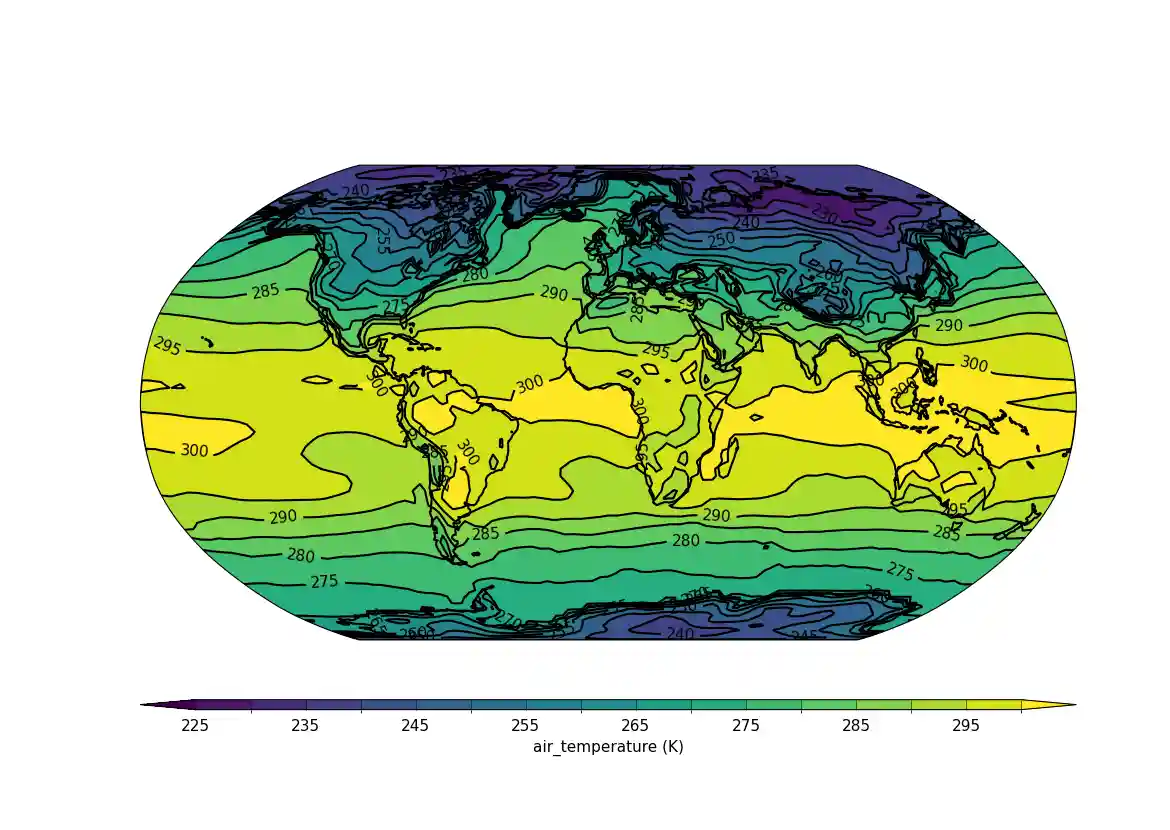
Example 38: Robinson projection#
Plotting using the Robinson projection#
f = cf.read(f"cfplot_data/tas_A1.nc")[0]

cfp.mapset(proj="robin")

cfp.con(f.subspace(time=15))